ARCHIVED – Chapter 4. Technology Case Results
This page has been archived on the Web
Information identified as archived is provided for reference, research or recordkeeping purposes. It is not subject to the Government of Canada Web Standards and has not been altered or updated since it was archived. Please contact us to request a format other than those available.
Content
- The Technology Case considers the impact of greater use of a selection of emerging energy technologies on the energy system. It builds upon the underlying assumptions of the HCP Case and the carbon price increases steadily throughout the projection period.
- The Technology Case assumes:
- Greater cost decreases for solar and wind electricity generating technology over the projection period.
- Greater interprovincial electricity trade and modest penetration of grid-scale battery storage technologies.
- Faster uptake of EVs in the passenger transportation sector.
- Higher adoption of steam-solvent technology in the oil sands sector.
- Greater electrification of space and water heating in the residential and commercial sectors.
- Increasing use of CCS technology for coal-fired electricity generation.
- These technologies are a selection of the wide array of emerging technologies that have the potential to increase their market share over the projection period. They are chosen to illustrate how technological development may impact energy supply and demand trends in various sectors of the economy. It is unclear which technologies will gain wider adoption in the future; these technologies provide an example among many potential outcomes. This sensitivity analysis is not a prediction or recommendation of certain technologies.
Technology Developments
- Over the past decade, technological changes have impacted the energy system in many ways. The widespread application of horizontal drilling and multistage hydraulic fracturing in tight and shale oil and natural gas resources was among the most impactful; significantly increasing production of crude oil and natural gas in North America.
- Other technological developments over the past decade have also influenced energy trends and have the potential to alter the long-term energy outlook in both Canada and globally. The following section discusses the specific technologies included in the Technology Case and is followed by a discussion of the energy supply and demand results.
Renewable Electricity Generation
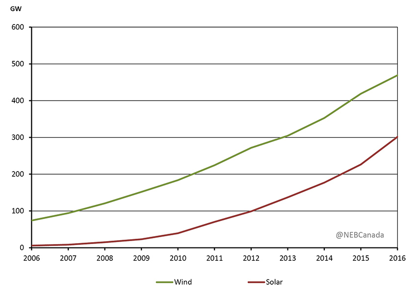
- Installations of renewable electricity generation technologies, particularly photovoltaic solar and wind, have increased significantly around the world over the past decade. Figure 4.1 shows cumulative global installations of solar photovoltaic and wind capacity.
Figure 4.1 - Cumulative Global Installed Solar Photovoltaic and Wind Generation Capacity
Description
This graph shows the cumulative global growth in installed solar photovoltaic and wind generation capacity from 2006 to 2016. From 2006 to 2016, wind generation capacity increased from 74 008 GW to 468 989 GW, while solar generation capacity increased from 5 762 GW to 301 473 GW.
Source: BP 2017 Statistical Review of World Energy
- A total of 1.5 GW of solar was installed globally during 2006 compared to more than 75 GW in 2016. China installed the most solar in 2016, followed by the U.S. and Japan. A total of 11 GW of wind was installed in 2006, compared to 55 GW in 2016.
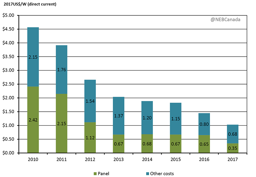
- Accompanying the increasing use of these technologies has been a decline in costs, particularly for solar photovoltaic installations. Figure 4.2 shows the estimated costs associated with a utility-scale solar installation in the U.S. from 2010 to 2017. Total installed costs fell from nearly US$4.5 per watt in 2010 to nearly US$1 per watt in 2016.
Figure 4.2 - U.S. Solar Photovoltaic Utility-Scale Solar System Cost Benchmark
Description
This chart breaks down the declining costs of utility scale solar generation, from 2007 to 2017, into the costs of the solar panel, and other associated costs. From 2010 to 2017, the costs of the solar panel fell from 2.42 US$/W (direct current) to 0.35 US$/W (direct current). Other associated costs also fell from 2.15 US$/W (direct current) in 2010, to 0.68 US$/W (direct current) in 2017. Overall, costs fell from 4.57 US$/W (direct current) in 2010, to 1.03 US$/W (direct current) in 2017.
Source: National Renewable Energy Laboratory (NREL)
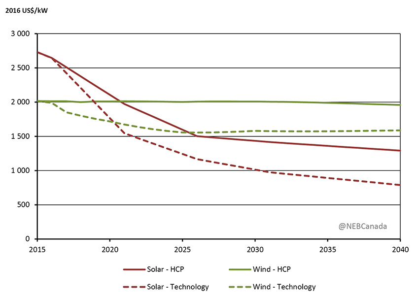
- Most industry observers expect the costs for solar and wind generation to continue to decline. The Technology Case assumes that these costs decline more steeply than in the Reference or HCP cases. Figure 4.3 shows the cost assumptions for solar (alternating current) and wind in the HCP and Technology cases.
Figure 4.3 - Capital Costs for Onshore Wind and Utility-Scale Solar Photovoltaic, HCP and Technology Cases
Description
This graph shows projected capital costs for onshore wind and utility-scale solar photovoltaic, under both the HCP and Technology Cases. Solar capital costs are 2 730 $US/kW in 2015, and by 2040 decrease to 1 290 $US/kW in the HCP case and 788 $US/kW in the technology case. Wind capital costs are 2 016 $US/kW in 2015, and by 2040 decrease to 1 958 $US/kW in the HCP case and 1 587 $US/kW in the technology case.
Source: NREL, Energy Information Administration (EIA)
Improving the Integration of Intermittent Renewables
- Electricity grid operators must constantly keep electricity production and consumption in balance to ensure the system is stable and reliable. Energy consumption changes continuously as demand from homes, businesses, and industry vary constantly. Electricity system operators’ main tool to keep the system in balance is to increase or decrease electricity generation to meet demand. Flexible generation resources, such as some hydroelectric and natural gas-fired facilities, are most often used to balance supply and demand for electricity.
- Unlike traditional generation sources, wind and solar are intermittent. They generate power when the wind is blowing or sun is shining. This can add to the challenge of balancing supply and demand because, in addition to fluctuations in electricity consumption, grid operators also need to accommodate variations in supply from these resources.
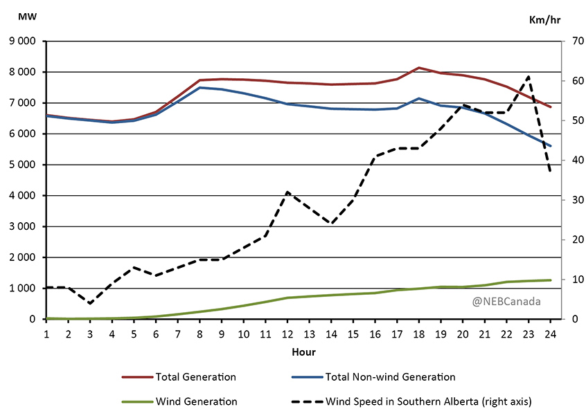
- Figure 4.4 shows an example of hourly generation in Alberta for a day in autumn 2015, a day with a large swing in wind generation. In the early hours of the day, almost all generation was from non-wind sources, primarily coal. Generation increased from 5:00 am to 8:00 am as homes and businesses increased their electricity use. Throughout the day wind speeds steadily increased, resulting in higher wind generation and lower non-wind generation. Later in the evening, total demand decreased while wind generation continued to increase. Wind was less than 1% of total generation in the morning and over 18% by midnight. This variability was accommodated by changes in output from other supply sources.
Figure 4.4 - Alberta Hourly Net to Grid Electricity Generation and Wind Speed, November 10, 2015
Description
This graph shows Alberta's hourly net to grid electricity generation and windspeed, for the day of November 10, 2015. The hourly windspeed was 8 km/hr beginning at hour 1 and steadily increases throughout the day, rising to 32 km/hr by hour 12 and ending at 37 km/hr by hour 24. Wind generation was 28 MW at hour 1 and slowly increases during the day, ending 1 264 MW by hour 24.
Source: Alberta Electric System Operator, Environment and Climate Change Canada
- When the share of intermittent resources is small, or if a grid has large levels of flexible generation available, fluctuations in supply are relatively easy to accommodate. However, as the shares of these resources increases, additional measures to accommodate increasing variability may be needed. These measures include:
- Building additional flexible generating capacity, such as natural gas-fired facilities, that can increase or decrease generation quickly.
- Various options to manage electricity demand, such as grid operators coordinating with large electricity users to increase or decrease their electricity use.
- Increasing transmission interconnections between electricity grids to allow greater electricity trade to manage variability.
- Building grid-scale electricity storage facilities that would charge and discharge to help balance the electricity system. Grid-scale storage includes many technologies such as pumped hydro, batteries, compressed air and flywheels.
- Compared to the Reference and HCP cases, the Technology Case assumes lower costs and modest penetration of grid-scale lithium ion batteries, greater use of demand management, and the expansion of the existing electricity interconnection between Alberta and B.C. by 500 MW.
Electric Vehicles
- The vast majority of vehicles on the road today utilize internal combustion engines (ICE) which are powered by fossil fuels, usually gasoline or diesel. EVs are powered by electricity stored in a battery and use an electric motor to propel the vehicle.
- EVs can include pure electric or hybrid vehicles. Pure electric EVs are only powered by an electric motor and the battery pack is charged by plugging into the electricity grid. Hybrids are vehicles that combine EV and ICE technologies. Plug-in hybrids have a battery that can be charged via the electricity grid but when the battery is depleted a small onboard ICE charges the battery to extend the vehicle’s range.
- As a passenger transportation vehicle, EVs have benefits and drawbacks compared to ICE vehicles. EVs have no tailpipe emissions, meaning they do not directly emit GHGs. However, if the electricity used to charge an EV is produced with fossil fuels, there would be GHG emissions associated with operating the vehicle. In some jurisdictions where coal is the dominant electricity source, charging an EV may result in more GHGs per kilometre driven compared to a similar sized ICE vehicle.
- Currently, the selection of EVs is growing but limited compared to ICE vehicles. EVs are also generally more expensive to purchase, largely as a result of battery pack costs. However, EVs are usually less expensive to drive per kilometre. This is partly due to higher efficiency of electric motors compared to ICEs and typically lower costs of electricity relative to gasoline or diesel in many provinces.
- One challenge with EVs can be the range of the vehicle, which can impact their usefulness for taking longer trips. The range of EVs are generally less than ICE vehicles although some with larger battery packs have comparable ranges. However, ICE vehicles have access to a well-established infrastructure of service stations to quickly refuel, accommodating trips further afield. EVs can take longer to charge, ranging from 30 minutes to many hours depending on the type of charger. Publically available charging stations are less common than refueling stations but their numbers are growing quickly. Table 4.2 compares some key characteristics of various electric vehicles and a typical ICE vehicle (Toyota Corolla).
Table 4.1 - Select Light Duty Vehicle Characteristics, 2017 Models
| Model | Range (km) | Purchase Price (US$) | KW.h/100 km | L/100km |
|---|---|---|---|---|
| Nissan Leaf | 172 | 33 735 | 30 | 2.1 |
| Ford Focus Electric | 185 | 29 120 | 31 | 2.2 |
| Hyundai Ioniq Electric | 200 | 31 000 | 25 | 1.7 |
| Volkswagen e-Golf | 201 | 32 295 | 28 | 2.0 |
| Chevrolet Bolt EV | 383 | 38 763 | 28 | 2.0 |
| Tesla Model X2 | 397 | 108 440 | 37 | 2.6 |
| Tesla Model S2 | 433 | 83 863 | 34 | 2.3 |
| Toyota Corolla (ICE) | 658 | 20 590 | - | 7.6 |
Source: Environmental Protection Agency
- Sales of EVs have increased in recent years due to a wider selection of vehicles, declining purchase costs and government policies aimed at increasing EV ownership. Figure 4.5 shows global annual sales of EVs, including plug-in hybrids. Total EVs on the road globally reached 2 million in 2016.
Figure 4.5 - Annual EV Sales, Pure and Plug-in Hybrid EVs
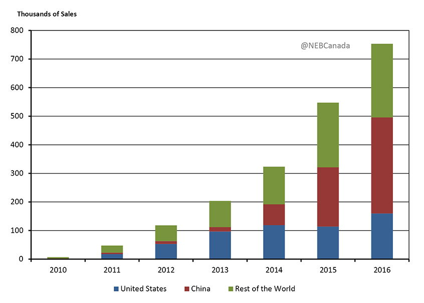
Description
This graph shows annual EV sales for both pure and plug-in hybrid EVS. Sales are shown for the United States, China, and the rest of the world. In 2010 annual sales were 1 190, 1 430 and 4 160 for each of the respective regions. By 2016 sales had risen to 159 000, 336 000 and 257 000, respectively.
Source: International Energy Agency
- EV sales in Canada, including plug-in hybrids, were 11 500 in 2016. This was 0.6% of all passenger vehicle sales in Canada in 2016.
- The Reference and HCP cases assume moderate market penetration of EVs, with the share of light duty vehicle annual sales reaching 3% in 2020 and 16% in 2040. Sales are stronger in regions of Canada that produce a large amount of their electricity from non-emitting sources and have EV policies. Sales grow quickest in Quebec as a result of the province’s EV mandate.
- The Technology Case assumes that recent growth in EV sales continue to accelerate, with lower battery costs and longer ranges encouraging greater adoption both globally and in Canada. The Technology Case assumes annual EV sales of 6% of total sales in 2020, and 47% in 2040. EVs gain a larger share in the passenger car market initially but also gain some share of the utility vehicle, light truck, and bus market later in the projection period. The Technology Case does not assume widespread adoption of autonomous driving technologies. Figure 4.6 shows the EV sales assumptions in the HCP and Technology cases.
Figure 4.6 - EV Share of New Passenger Vehicle Purchases, HCP and Technology Cases
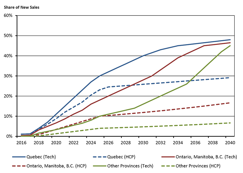
Description
This graph shows EV share of new vehicle purchases under both the HCP and Technology Case for solely Quebec, as well as Ontario, Manitoba and B.C. together, and then the remaining provinces. In 2016, the EV shares of new vehicle purchases are 1.08% in Quebec, 0.42% for Ontario, Manitoba, and B.C., and 0.11% for the remaining provinces. Under the HCP Case, these values grow to 29.15%, 16.67% and 6.67% by 2040. Under the Technology Case, the values grow to 48%, 46.50% and 45%.
- In the HCP Case, roughly 16% the passenger vehicles on the road in 2040 are EVs, or about 3 million vehicles. In the Technology Case, there are approximately 8 million EVs on the road in 2040, or about 34% of all passenger vehicles.
Steam-Solvent Technology in the Oil Sands
- Extracting bitumen from the oil sands can be energy intensive, particularly for in situ operations. In situ oil sands production involves burning natural gas to create steam, which is then injected into reservoirs to reduce the viscosity of the bitumen, allowing it to be pumped to the surface. In recent years, technology and process improvements have reduced the amount of steam, and hence natural gas, used per barrel. Further discussion of this trend is available in the “Energy Use in the Oil Sands” section in Chapter 2 of Canada’s Energy Future 2016.
- The decline in crude oil prices since mid-2014 — along with the implementation of carbon pricing and a 100 MT cap on oil sands emissions — creates an incentive for oil sands producers to continue to reduce costs and GHG emissions. Many different technologies are being proposed and tested in the oil sands. Steam-solvent processes are one technology that has potential to reduce in situ supply costs, natural gas consumption, and GHG emissions.
- Steam-solvent processes involve combining solvents, such as propane or butane, with the steam being injected into in situ reservoirs. Solvent concentrations in the steam can range from 10% to 20%. The addition of solvents aids in reducing the viscosity of the bitumen in the reservoir and has shown to improve recovery rates from wells by 10% to 30% compared to steam alone. The technology also has potential to reduce the energy intensity of production considerably. Steam-solvent processes differ from pure solvent processes, which involve using only solvents to extract bitumen.
- An in situ project using steam-solvent technology can have higher upfront costs than a traditional in situ project as a result of additional facilities to store, treat, and recover solvents. Greater bitumen recovery rates and lower steam requirements can offset those costs to varying extents depending on individual project characteristics. The economics of steam-solvent processes are influenced by the cost of the propane or butane to be injected. In recent years the price of these commodities, particularly propane, have been quite low due to increasing production of liquids-rich tight and shale gas in western Canada. Another factor in the cost effectiveness of steam-solvent processes is the extent to which the injected solvents can be recovered from the reservoir. Typical recovery rates are around 70% but can vary widely.
- Several pilot projects have successfully implemented steam-solvent technology and some commercial scale projects are under consideration. Cenovus stated that its Narrows Lake project, which was recently deferred due to low oil prices, would employ steam-solvent technology on a commercial scale. Imperial Oil’s Aspen and Cold Lake expansion projects both propose to apply steam-solvent processes and are currently under regulatory review.
- The Technology Case assumes that oil sands producers increasingly use steam-solvent processes. Early in the projection period, the technology is applied at select expansion projects and is gradually implemented at existing facilities later in the projection period. Higher oil recovery rates and lower steam requirements reduce the cost per barrel of building new or expanding in situ facilities by roughly 30%. For existing facilities, bitumen recovery rates increase and natural gas consumption declines as a result of the use of steam-solvent processes.
Greater Electrification of Space and Water Heating
- Several different technologies are used to heat homes and businesses in Canada. Most are heated using natural gas or oil furnaces, electric baseboard heating or with wood. The predominant type of heating in a region is usually determined by the relative costs of fuels and the infrastructure to deliver those fuels. For example, low electricity prices in Quebec encourages more electric baseboard heating. In Atlantic Canada, oil furnaces and electric heat are more common, in part due to limited natural gas distribution infrastructure. Figure 4.7 demonstrates the heating system types across Canada.
Figure 4.7 - Share of Residential Heating System Type by Region, 2014
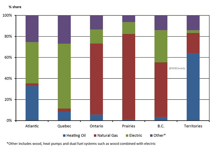
Description
This graph shows the share of residential heating system type by region, for the year of 2014. The four residential system heating types are heating oil, natural gas, electric and other. In Atlantic Canada heating oil accounted for 33% of residential heating systems, while natural gas accounted for 2.5%, electric accounted for 39%, and other sources accounted 25%. In Quebec, heating oil accounted for 8.5% of residential heating systems, while natural gas accounted for 3%, electric accounted for 61% and other heating systems accounted for 27%. In Ontario, heating oil accounted for 6% of residential heating systems, while natural gas accounted for 81%, electric accounted for 11%, and other heating systems accounted 6.3%. In The Prairies, heating oil accounted for 1.3% of residential heating systems, while natural gas accounted for 81%, electric accounted for 11% and other heating systems accounted for 6.3%. In B.C., heating oil accounted for 3.4% of residential heating systems, while natural gas accounted for 51%, electric accounted for 31% and other heating systems accounted for 14%. In The Territories, heating oil accounted for 64% of residential heating systems, while natural gas accounted 19%, while electric accounted for 2.6% and other heating systems accounted 14%.
Source: Natural Resources Canada
- The energy efficiency and GHG intensity of space and water heating depends on a variety of factors, including heating system type, the quality of a building’s insulation and weather sealing, type of heating fuel, and local climate conditions.
- Heat pumps operated with electricity are an alternative technology that can be used for space and water heating. Heat pumps use similar processes as freezers or air conditioners but can heat a space rather than cool it. Most heat pumps can both heat and cool as needed.
- The advantage of heat pumps is that rather than directly creating heat, they exchange energy, extracting heat from an outside source and pumping it into a space. As a result, a heat pump uses two to five times less electricity compared to baseboard heating to generate the same amount of heat. The efficiency of a heat pump depends on the temperature of the medium it is extracting heat from — the lower the temperature, the more energy it takes to extract the heat.
- There are two main types of heat pumps: air and ground source. Air source heat pumps extract heat from the air outside. Ground source heat pumps are typically part of a geo-exchange system, where the heat is extracted from a liquid that is pumped through underground pipes which either absorb or dissipate heat to and from the ground.
- The Technology Case assumes heat pumps installations increase to 15% of new heating device purchases in 2025, for both new buildings and retrofits in existing buildings. The share of installations increase to 30% by 2040.
CCS Technology
- CCS technology involves capturing and storing CO2 emissions that would have otherwise been released into the atmosphere. The carbon is usually stored underground in geological formations. CCS projects are usually designed to capture CO2 from large sources of emissions, such as power plants or natural gas processing plants, to take advantage of concentrated streams of GHG emissions. Global large scale CCS capacity was 34 MT in 2016, which is equivalent to about 5% of Canada’s GHG emissions.
- Carbon can be captured using a variety of processes. Pre-combustion processes convert fossil fuels to hydrogen and CO2. The hydrogen can then be used for energy or other processes and the CO2 stored. Post-combustion processes involve separating CO2 from the exhaust from an industrial facility or power plant using a variety of techniques. There are also oxy-fuel processes involving combusting fossil fuels in an oxygen-rich environment, resulting in an exhaust stream of mostly water and CO2, making it easier to recover a concentrated CO2 stream suitable for storage.
- In many cases, the CO2 stream resulting from CCS is used for other purposes. One common use is for enhanced oil recovery (EOR), where CO2 is injected into oil-bearing reservoirs to increase the amount of oil that can be extracted.
- The Boundary Dam power station in Saskatchewan began operations in 2014. The 115 MW coal-fired power plant is capable of capturing 1.3 MT of CO2 per year. Most of the CO2 from the facility is transported to nearby oil fields and used for EOR while some is also stored underground in geological formations near the plant. In addition, Saskatchewan has also been importing CO2 by pipeline for EOR from a coal gasification plant in North Dakota.
- In Alberta, the Quest Project captures CO2 from Shell’s Scotford upgrader and transports it by pipeline for permanent storage underground. The project is designed to capture up to 1.1 MT of CO2 per year or roughly 35% of the upgrader’s emissions. Under development is the Alberta Carbon Trunk Line, a 240 km pipeline that will transport CO2 from an industrial area north of Edmonton to EOR projects in central Alberta. Starting in 2018 the project will transport 1.7 MT CO2 per year captured from two facilities: the Sturgeon Refinery (currently under construction) and an Agrium fertilizer plant. The pipeline has a capacity of nearly 15 MT per year to allow for future CCS projects.
- The Reference and HCP cases include some additional CCS projects over the projection period. This includes the retrofitting of the additional coal units at Boundary Dam in Saskatchewan, with units 4 and 5 coming online in 2021 and unit 6 coming online in 2029. The Technology Case assumes that ongoing research and development in CCS technology results in lower costs and encourages more CCS capacity to be added over the projection period. This includes retrofitting Boundary Dam unit 6 with CCS earlier and additional retrofits of the existing coal-fired generation facilities in Saskatchewan and Alberta. Figure 4.8 shows total installed capacity of coal-fired generation with CCS technology installed.
Figure 4.8 - Installed Coal-Fired Generation Capacity with CCS, HCP and Technology Cases
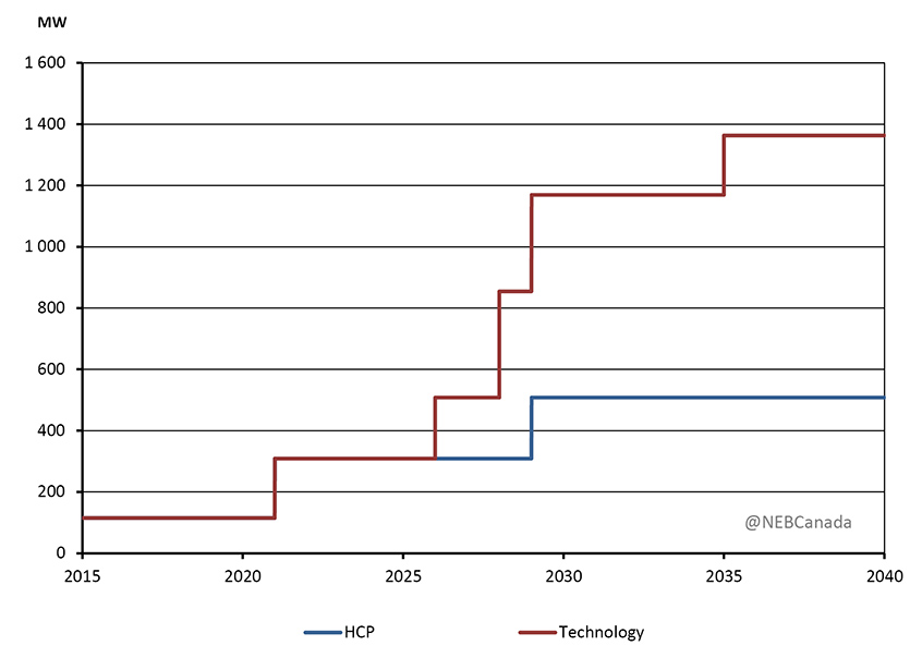
Description
This line graph shows installed coal-fired generation capacity with CCS, under both the HCP and Technology Cases. In 2015 there was 115 MW of coal-fired generation capacity with CCS. By 2040 this value increases to 558 MW under the HCP Case, and to 1363 MW under the Technology Case.
Technology Case Results
- The Technology Case builds upon the underlying assumptions of the HCP Case, meaning the carbon price increases steadily throughout the projection period. As noted in Chapter 2, the Technology Case assumes that greater adoption of technologies like electric vehicles has an impact on global crude oil demand. As a result, the crude oil price is lower than in Technology Case compared to the HCP or Reference cases, reaching US$65/bbl in 2040.
Macroeconomic Drivers
- Key economic variables are shown in Table 4.1. Economic growth averages 1.74% per year over the projection period in the Technology Case, slightly higher than in the Reference Case.
Table 4.2 - Economic indicators, Reference, HCP and Technology Cases, 2016-2040
| Economic Indicator | Compound Average Annual Growth Rate (unless otherwise noted) | ||
|---|---|---|---|
| Reference Case | HCP Case | Technology Case | |
| Real Gross Domestic Product | 1.73% | 1.72% | 1.74% |
| Population | 0.76% | 0.76% | 0.76% |
| Exchange Rate (average) | 83.7 US/C$ | 83.4 US/C$ | 82.0 US/C$ |
- Lower crude oil prices and production in the Technology Case depreciate the Canadian-US exchange rate relative to the other cases. This, along with reduced energy costs due to the various technologies in the Technology Case, leads to faster economic growth. However, the overall economic outcomes in all three cases are similar, despite shifts in the energy system. By 2040, gross domestic product is 0.2% lower in the Higher Carbon Price Case than in the Reference Case, and 0.1% higher in the Technology Case.
Residential, Commercial, and Transportation Energy Demand
- The technologies considered in the Technology Case impact energy use in a variety of ways, and result in a decrease in end-use energy demand. Total end-use demand in 2040 in the Technology Case is 11 045 PJ, or 2.6% lower than in the HCP Case and 9% lower than in the Reference Case.
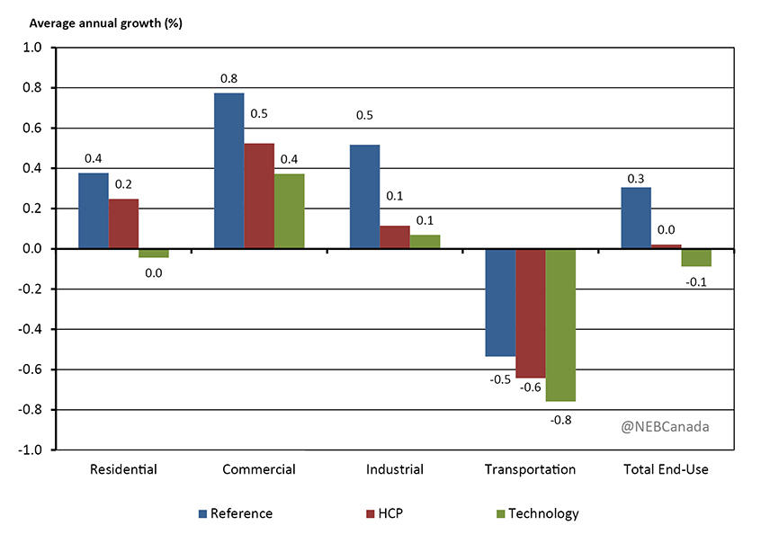
- Figure 4.9 shows average annual growth rates for total end-use demand as well as the four sectors. Energy use grows more slowly or declines faster than the HCP Case. These trends are a result of the specific technology assumptions in the Technology Case, as well as the impacts of lower crude oil prices and changing macroeconomic drivers.
Figure 4.9 - Projected Annual Average Growth in End-Use Energy Demand by Sector, 2016 to 2040, All Cases
Description
This graph shows the projected annual average growth in end-use energy demand by sector, under both the reference, HCP, and Technology cases. Under the Reference Case the average annual growth rate for the residential sector is 0.4%, 0.8% for the commercial sector, 0.5% for the industrial sector, -0.5% for the transportation sector, and 0.3% for total end use. Under the HCP Case, the average annual growth rate for the residential sector is 0.2%, 0.5% for the commercial sector, 0.1% for the industrial sector, -0.6% for the transportation sector, and 0% for total end use. Under the Technology Case the average annual growth rate for the residential sector is 0%, 0.4% for the commercial sector, 0.1% for the industrial sector, -0.8% for the transportation sector, and -0.1% for total end use.
Residential and Commercial
- The higher penetration of heat pumps for heating and cooling in buildings leads to lower energy use in the residential and commercial sector because that technology heats and cools more efficiently than conventional natural gas, electric, or oil systems.
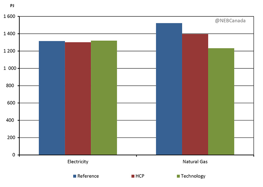
- Figure 4.10 compares residential and commercial electric and natural gas demand in 2040 across the cases. Electricity demand increases slightly in the Technology Case. Greater electrification of heating is partially offset by improving the energy efficiency of heating in jurisdictions such as Quebec that have a high share of electric baseboard heating. Greater electrification reduces natural gas demand in buildings, which is 12% lower in the Technology Case compared to HCP Case.
Figure 4.10 - Residential and Commercial Electricity and Natural Gas Demands in 2040, All Cases
Description
This graph shows electricity and natural gas demand in 2040 for the residential and commercial sectors combined, under each of Reference, HCP and Technology Cases. Under the Reference Case, electricity demand is 1 315 PJ and natural gas demand is 1 522 PJ. Under the HCP Case, electricity demand is 1 301 PJ and natural gas demand is 1 396 PJ. Under the Technology Case, electricity demand is 1 319 PJ and natural gas demand is 1 232 PJ.
Transportation
- An increased share of electric vehicles reduces transportation energy demand in the Technology Case. Total transportation energy demand in the Technology Case is 3% lower than HCP and over 5% lower than the Reference Case in 2040. Demand is lower because electric vehicles typically use less energy per km travelled compared to conventional vehicles. This impact is muted however due to the lower oil price assumption in the Technology Case. The resulting lower gasoline and diesel prices encourage more driving by the remaining conventional gasoline and diesel vehicles.
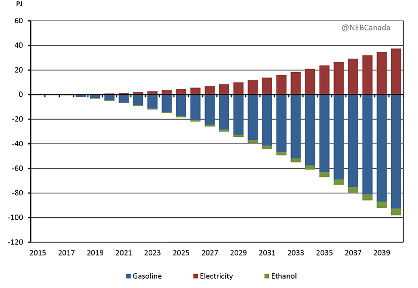
- Figure 4.11 shows the difference in demand between the Technology and HCP cases for electricity, gasoline, and ethanol, which is blended with gasoline. As the share of electric vehicles in transportation grows, electricity demand increases, offsetting use of gasoline and blended ethanol. In 2040, electricity demand is 37 PJ higher than in the HCP case, and gasoline demand is reduced by 98 PJ.
Figure 4.11 - Difference in Electricity, Gasoline and Ethanol Use between the Technology and HCP Cases
Description
This bar graph shows the net difference in demand, by fuel, between the Technology and HCP cases. By 2040, the difference in gasoline demand is -93 PJ, the difference in electricity demand is 37 PJ and the difference in ethanol demand is -6 PJ.
- In the Technology Case, ethanol is blended with gasoline according to minimum federal and provincial blending requirements. As a result of lower gasoline use, ethanol use is 5.5 PJ lower in 2040 in the Technology Case compared to the HCP Case.
Crude Oil Production and Industrial Energy Demand
- In the Technology Case, oil sands producers increasingly use steam-solvent technologies for in situ projects. This reduces the per barrel costs for new projects and expansions of existing projects. However, the Technology Case also assumes that greater technological adoption occurs globally, reducing crude oil consumption overall. As a result, crude oil prices in the Technology Case are lower, reaching US$65/bbl in 2040 compared to US$75/bbl in the HCP Case and US$80/bbl in the Reference Case. Lower supply costs are partially offset by the lower price assumptions in the Technology Case and production reaches 416 103m3/d (2.6 MMb/d) by 2040, 3% higher than in the HCP Case.
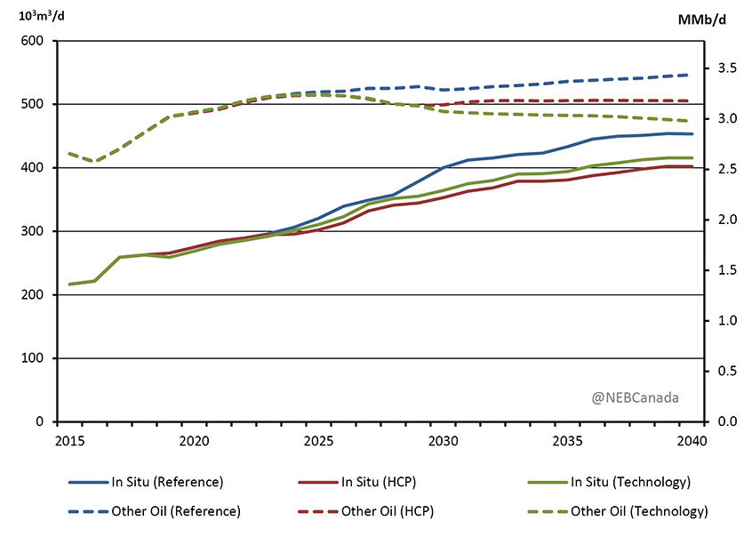
- The costs of production for conventional and mined oil sands resources do not decrease significantly in the Technology Case. Mined oil sands production is the same as no new production is added beyond those facilities currently under construction in all three cases. Conventional oil production, including offshore Newfoundland and Labrador production, is lower in the Technology Case as result of lower price assumptions. Figure 4.12 shows in situ oil sands and all other crude oil production in all three cases.
Figure 4.12 - In Situ and Other Crude Oil and Equivalent Production, All Cases
Description
This graph shows the projected in-situ and all other crude oil production under each of the Reference, HCP, and Technology cases. In 2015 in-situ production was 217 103m3/day. By 2040, in situ production is 453 103m3/day, 402 103m3/day and 416 103m3/day, under the Reference, HCP and Technology Cases, respectively. In 2015 all other oil production is 422 103m3/day. By 2040, all other production is 547 103m3/day, 505 103m3/day and 473 103m3/day, under the Reference, HCP and Technology cases, respectively.
- The use of steam-solvent technology in the Technology Case reduces the amount of steam, and hence natural gas, used per barrel of production. Figure 4.13 shows production-weighted SOR in all three cases. Higher in situ production in the Technology Case is more than offset by lower SORs, and in situ oil sands energy demand is 6.5% lower than the HCP Case in 2040.
Figure 4.13 - Annual Average Production-Weighted Steam Oil Ratio of Thermal Oil Sands Production, All Cases
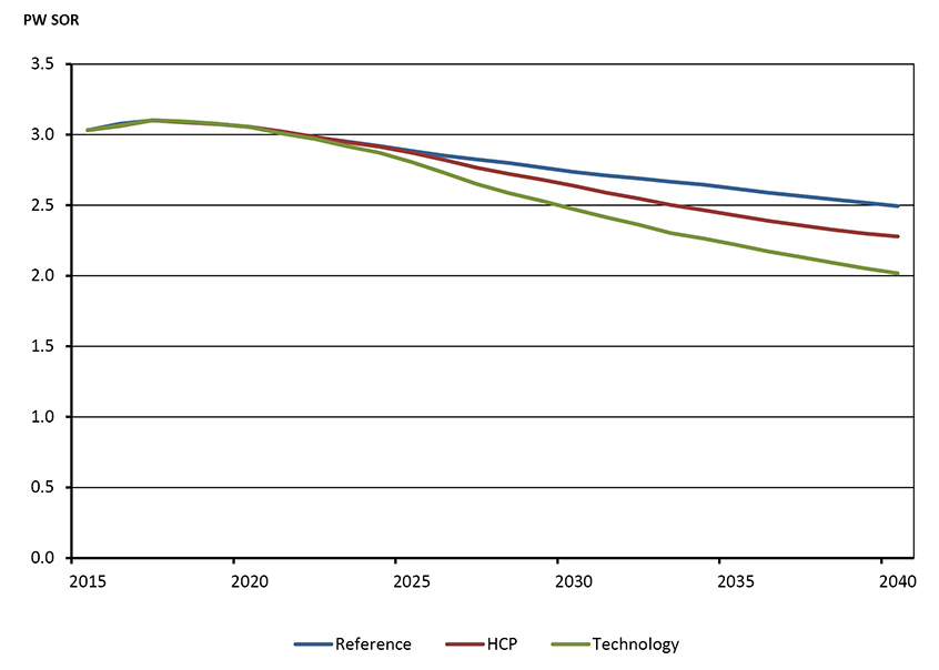
Description
This graph shows the projected annual average production weighted (PW) improvements in the steam oil ratio (SOR) of thermal oil sands productions, for the Reference, HCP and Technology Cases. In 2015 the PW SOR was 3.03, by 2040 the PW SOR is 2.5, 2.27 and 2.02 under the Reference, HCP and Technology cases, respectively.
- Natural gas production is 3% lower in the Technology Case compared to the HCP Case in 2040. This is primarily because lower crude oil production results in lower production of solution gas, the natural gas produced along with oil from oil wells.
- Overall industrial energy use in the Technology Case is 1% lower than the HCP Case in 2040. Lower oil sands energy use in the Technology Case is offset by slightly higher energy use in other sectors. This is largely a result of higher economic growth in some export-oriented industries and lower energy price assumptions relative to the HCP Case, which decrease end-use energy prices and increase demand.
Electricity
- Although total end-use demand is lower in the Technology Case, a shift towards electricity in buildings and transportation causes electricity demand in the Technology Case to be 2.7% higher than the HCP Case in 2040. This, combined with lower renewable costs, increased CCS, and improved integration of renewable sources leads to a shift in the electricity mix in the Technology Case.
- By 2040, total capacity in the Technology Case is 8.8% higher than the HCP Case, and 40% higher than 2015 levels. Due to lower costs and measures to improve the integration of renewables, solar capacity in 2040 is 16 GW higher in the Technology Case relative to HCP Case, and wind capacity is 4.4 GW higher. In the Technology Case, wind and solar make up 27% of Canada’s capacity mix in 2040, compared to 19% in the Reference and HCP cases, and 9% in 2015. Figure 4.14 shows total electric capacity by fuel in 2015 and 2040 in all three cases.
Figure 4.14 - Generating Capacity by Fuel, 2015 and 2040, All Cases
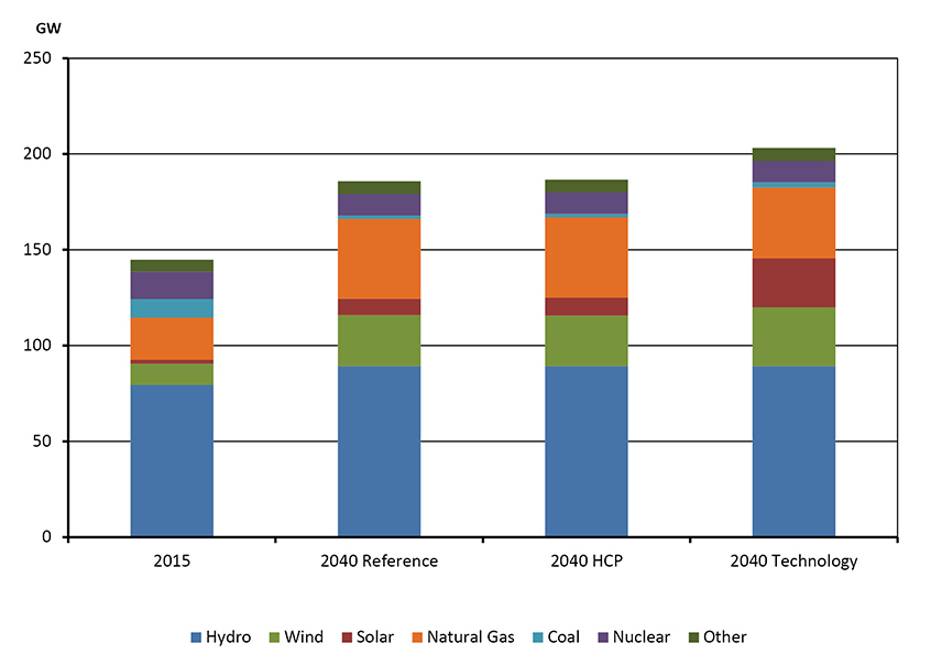
Description
This graph shows generating capacity by fuel in 2015 and 2040 for the Reference, HCP, and Technology cases. In 2015 the respective generating capacity for hydro, wind, solar, natural gas, coal, nuclear and other fuels was 79.43 GW, 11.07 GW, 2.13 GW, 22.00 GW, 9.66 GW, 14.27 GW and 6.26 GW. In 2040 under the Reference Case the respective generating capacity for hydro, wind, solar, natural gas, coal, nuclear and other fuels is 89.25 GW, 26.60 GW, 8.5 GW, 41.72 GW, 1.78 GW, 11.11 GW and 6.78 GW. In 2040 under the HCP Case the respective generating capacity for hydro, wind, solar, natural gas, coal, nuclear and other fuels is 89.25 GW, 26.37 GW, 9.36 GW, 41.98 GW, 1.78 GW, 11.11 GW and 6.78 GW. In 2040 under the Technology Case the respective generating capacity for hydro, wind, solar, natural gas, coal, nuclear and other fuels is 89.25 GW, 30.79 GW, 28.49 GW, 37.08 GW, 2.64 GW, 11.11 GW and 6.77 GW.
- Natural gas capacity does not grow as fast in the Technology Case, but still increases relative to current levels. In 2040, natural gas capacity in the Technology Case is nearly 70% higher than in 2015, as it continues to play an important role in replacing retired coal capacity and balancing intermittent renewables. Additional CCS capacity in Alberta and Saskatchewan increases the share of coal-fired capacity compared to the Reference and HCP cases.
- Electricity generation is 3% higher in the Technology Case compared to the HCP Case in 2040. This is less than the 8% increase in capacity because most of the additions are wind and solar. These resources are variable depending on wind speeds and sun intensity, and over the course of a year tend to generate less per megawatt of capacity compared to other sources of electricity. While wind and solar make up 27% of the capacity mix in 2040, these resources account for 16.5% of generation. Figure 4.15 shows generation by select fuel in 2015 and 2040 in all cases.
Figure 4.15 - Generation by Select Fuels, 2015 and 2040, All Cases
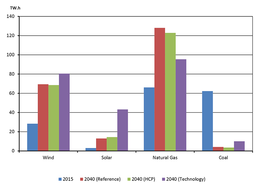
Description
This bar graph shows the generation by fuel in 2015 and 2040 for the Reference, HCP and Technology cases. In 2015 the respective generation for wind, solar, natural gas and coal was 28.3 TW.h, 3.0 TW.h, 66.1 TW.h and 62.3 TW.h. In 2040 under the Reference Case the respective generation for wind, solar, natural gas and coal is 69.38 TW.h, 12.98 TW.h, 128.05 TW.h and 4.14 TW.h. In 2040 under the HCP Case the respective generation for wind, solar, natural gas and coal is 68.56 TW.h, 14.40 TW.h, 122.81 TW.h and 3.50 TW.h. In 2040 under the Technology Case the respective generation for wind, solar, natural gas and coal is 80.49 TW.h, 43.22 TW.h, 95.37 TW.h and 10.06 TW.h.
- The shift towards wind, solar, and coal with CCS causes Canada’s already low emitting electricity sector to become even greener. The share of non-emitting resources increases to 86% in the Technology Case in 2040, compared to 82% in the Reference and HCP cases, and 80% in 2015.
GHG Emissions
- The Technology Case has implications for primary energy demand because of the shift towards more electricity and reduced overall demand in the end-use sector, and more renewable generation in the electricity sector. These changes further reduce Canada’s GHG emission trajectory, as less fossil fuels are combusted and more carbon is captured and sequestered.
- The Technology Case adds renewable and coal demand due to the shift in the electricity mix.
- Oil product demand declines primarily because of reduced consumption in the transportation sector. Natural gas demand declines relative to the HCP Case in the residential, commercial, and industrial end use sectors, as well as in electric generation.
Figure 4.16 - Change in Primary Energy Demand by Fuel Type, Technology Case vs HCP
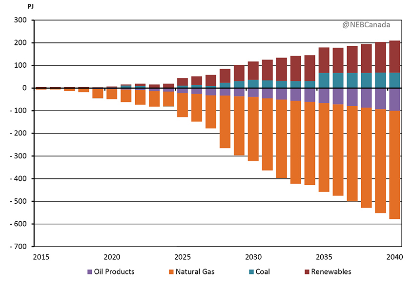
Description
This graph shows the net difference from 2015 to 2040 in primary energy demand between the HCP and Technology Case, broken down by fuel type. By 2020, oil product demand is 5.04 PJ lower in the Technology Case compared to the HCP Case, natural gas demand is 43.7 PJ lower in the Technology Case, coal demand is 2.34 PJ higher in the Technology Case, and renewables are 4.54 PJ higher. By 2030, oil product demand is 39.02 PJ lower in the Technology Case compared to the HCP Case, natural gas demand is 282.33 PJ lower in the Technology Case, coal demand is 36.52 PJ higher in the Technology Case, and renewables are 81.01 PJ higher. By 2040, oil product demand is 100.3 PJ lower in the Technology Case compared to the HCP Case, natural gas demand is 477.9 PJ lower in the Technology Case, coal demand is 68.2 PJ higher in the Technology Case, and renewables are 141.9 PJ higher.
- The impact of these changes causes total primary demand to decline in the Technology Case, both relative to the Reference and HCP projections, as well as 2015 values. By 2040, total primary demand in the Technology Case is 2.7% less than 2015 levels, 8.5% less than the Reference Case in 2040, and 2.9% less than the HCP Case in 2040.
- Total fossil fuel demand in the Technology Case declines faster than total primary demand. By 2040, total fossil fuel use in the Technology Case is 7.4% less than 2015 values, 13% less than the Reference Case in 2040, and 5% less than the HCP Case in 2040. Figure 4.18 shows the difference in fossil fuel use from the Reference Case for both the HCP and Technology cases.
Figure 4.17 - Total Fossil Fuel Use - Percentage Difference in the HCP and Technology Cases from the Reference Case
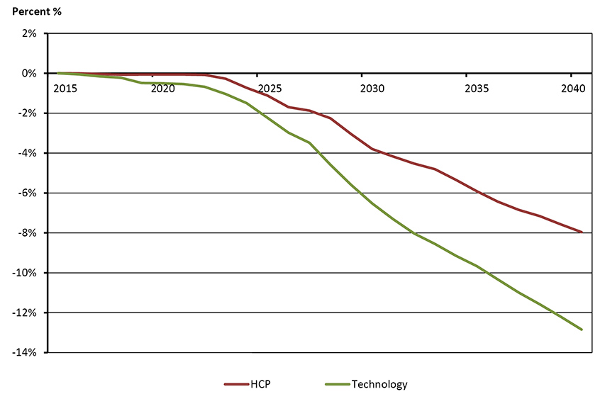
Description
This graph shows the percentage difference in total fossil fuel use from the Reference Case, for the HCP and Technology cases over the projection period. By 2020 the HCP Case is 0.1% lower than the Reference Case, while the Technology Case is 0.5% lower than the Reference Case. By 2030 the HCP Case is 3.8% lower than the Reference Case, while the Technology Case is 6.5% lower than the Reference Case. By 2040 the HCP Case is 8.0% lower than the Reference Case, while the Technology Case is 12.8% lower than the Reference Case.
- The GHG emission intensity of the fossil fuel mix in the Technology Case is similar to the Reference and HCP cases (Figure 4.18). Natural gas decreases more than other fuels in the Technology Case relative to the HCP Case, and because natural gas is less emissions-intensive than other fuels, this will increase the average CO2 per megajoule intensity. However, increases in carbon sequestration from CCS units in the Technology Case offset this effect and lead to lower emissions intensity. By 2040, emission intensity of the fossil fuel mix in the Technology Case is just 0.5% less than the HCP Case.
Figure 4.18 - Estimated Weighted-Average GHG Emission Intensity of Fossil Fuel Consumption, Reference, HCP and Technology Cases
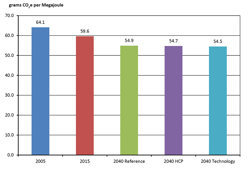
Description
This graph shows the estimated weighted average GHG emission intensity of fossil fuel consumption, for each of the Reference, HCP and Technology cases. In 2005 the emissions intensity was 64.1 grams CO2e per megajoule, and in 2015 energy intensity was 59.6 grams CO2e per megajoule. By 2040 the emissions intensity is projected to be 54.9 grams CO2e per megajoule in the Reference Case, 54.7 grams CO2e per megajoule in the HCP Case, and 54.5 grams CO2e per megajoule in the Technology Case.
- The analysis in Energy Futures 2017 presents projections of future energy demand and supply under various assumptions, and is not a pathway to meet specific climate goals or targets. As in the Reference and HCP cases, accounting for reductions in non-combustion emissions, such as reducing methane leaks, as well as including emission credits purchased through international trading mechanisms (such as Ontario and Quebec’s emission trading with California) could further decrease Canada’s emissions trajectory.
- The pace and magnitude of technological change is a key uncertainty in these projections, and the Technology Case explores this uncertainty by illustrating the impact of select technologies on the energy system. Numerous other technologies could be employed to further decarbonize Canada’s energy system. Likewise, the market response to the increased carbon price in the HCP and Technology cases could be higher or lower than what is projected.
- The HCP and Technology cases do not represent a ceiling on Canada’s potential for GHG emission reductions. Rather, the cases illustrate the impact climate policy and technology can have on Canada’s energy system. EF 2017 shows that both factors can bend Canada’s fossil fuel use trajectory in a meaningful way, and will influence the way Canadians produce and consume energy over the next several decades.
Key Uncertainties
- The Technology Case examines the impact of higher carbon prices as well as the increased adoption of select technologies in the long term. The impacts in this case are based on the suite of models and assumptions employed for this analysis. Other energy models or assumptions could produce different impacts of carbon pricing and technology trends.
- Numerous other emerging technologies could affect Canada’s energy system in the future. If the technologies explored here gain a significant market share in the future, the speed at which they are adopted could be faster or slower than assumed in the Technology Case. Energy transitions have happened many different ways in history, and the eventual path of future transitions could be much different than shown here.
- The impact of a global shift to greater climate policy action and broader adoption of low carbon technologies on global energy markets is highly uncertain. The HCP and Technology Cases assume that crude oil prices are lower than the Reference Case, but this impact could be smaller or larger. Natural gas, coal, and electricity markets could all be affected by changing global dynamics, as could the supply and demand for energy intensive goods. These changes will have implications for Canadian macroeconomic, energy and emission trends.
- The Technology Case shows a higher penetration of wind and solar electricity generation due to lower cost and improved integration. Both of these factors are important for the future of solar and wind in Canada. Costs could fall more or less than assumed in the Technology Case. Even with lower costs, challenges in integrating these intermittent resources could limit their uptake. Alternatively, advances in integrating wind and solar resources could lead to them making up an even higher share of Canada’s electricity mix than shown in the Technology Case.
- Date modified: