ARCHIVED – Natural Gas Supply Costs in Western Canada in 2009 – Energy Briefing Note
This page has been archived on the Web
Information identified as archived is provided for reference, research or recordkeeping purposes. It is not subject to the Government of Canada Web Standards and has not been altered or updated since it was archived. Please contact us to request a format other than those available.
ISSN 1917-506X
Natural Gas Supply Costs in Western Canada in 2009 - Energy Briefing Note [PDF 3848 KB]
Energy Briefing Note
November 2010
Copyright/Permission to Reproduce
List of Acronyms and Abbreviations
| Alberta NIT | Alberta NOVA Inventory Transfer |
| CBM | Coalbed Methane |
| CPI | Consumer Price Index |
| HSC | HSC Horseshoe Canyon |
| NEB | National Energy Board |
| NCF | Net Cash Flow |
| NGLs | natural gas liquids |
| NPV | Net Present Value |
| ROR | Rate of Return |
List of Units and Conversion Factors
| Units | |
|---|---|
| m³ | = cubic metres |
| MMcf | = million cubic feet |
| Bcf | = billion cubic feet |
| m³/d | = cubic metres per day |
| 10³m³/d | = thousand cubic metres per day |
| MMcf/d | = million cubic feet per day |
| Bcf/d | = billion cubic feet per day |
| GJ | = gigajoule |
Common Natural Gas Conversion Factors
1 million m³ (@ 101.325 kPaa and 15oC) = 35.3 MMcf (@ 14.73 psia and 60oF)
1 GJ (Gigajoule) = .95 Mcf (thousand cubic feet) = .95 MMBtu = .95 decatherms
Price Notation
Canadian natural gas prices are quoted as the Alberta NIT Gas Reference Price and are listed in $C/GJ.
Table of Contents
- Foreword
- Overview
- Methodology
- Results
- Observations
- Appendices
- Appendix 1 - Cost Factors
- Appendix 2 - Production and Cost Input Methodology
- Appendix 3 - Economic Methodology
- Appendix 4 - Formations
- Appendix 5 - Groupings
- Appendix 6 - Decline Parameters
- Appendix 7 - Gas Compositions
- Appendix 8 - Other Well Parameters
- Appendix 9 - Formation Ratios by Grouping
- Appendix 10 - 2009 Capital Cost
- Appendix 11 - 2009 Operating and Processing Costs
- Appendix 12 - 2009 Rate of Return
- Appendix 13 - 2007 versus 2009 Comparison of Key Values
- Appendix 14 - 2009 Supply Cost Components
Foreword
The National Energy Board (the Board) is an independent federal organization established in 1959 to promote safety and security, environmental protection and economic efficiency in the Canadian public interest[1] within the mandate set by Parliament for the regulation of pipelines, energy development and trade.
[1] The public interest is inclusive of all Canadians and refers to a balance of economic, environmental, and social interests that change as society's values and preferences evolve over time. As a regulator, the Board weighs the relevant impacts on these interests when making its decisions.
The Board's main responsibilities include regulating the construction, operation and abandonment of interprovincial and international oil and gas pipelines, international power lines, and designated interprovincial power lines. Furthermore, the Board regulates the tolls and tariffs for the pipelines under its jurisdiction. With respect to the specific energy commodities, the Board regulates the export of natural gas, oil, natural gas liquids (NGLs) and electricity, and the import of natural gas. Additionally, the Board regulates oil and gas exploration and development on frontier lands and offshore areas not covered by provincial or federal management agreements.
In an advisory function, the Board reviews and analyzes matters related to its jurisdiction and provides information and advice on aspects of energy supply, transmission and disposition. In this role, the NEB publishes periodic assessments to inform Canadians on trends, events, and issues that may affect Canadian energy markets.
This report is an energy briefing note - a brief report covering one aspect of energy commodities. This report analyzes the supply costs of developing natural gas in Western Canada in 2009. It is the second edition covering this topic, following the 2007 supply cost report released in August 2008.[2]
[2] Natural Gas Supply Costs in Western Canada in 2007 - Energy Briefing Note
In preparing this report, the NEB gained valuable feedback on well inputs, specifically cost information, from various producers. The NEB appreciates the information and comments provided and would like to thank all participants for their time and expertise.
If a party wishes to rely on material from this report in any regulatory proceeding before the NEB, it may submit the material, just as it may submit any public document. Under these circumstances, the submitting party in effect adopts the material and that party could be required to answer questions pertaining to the material.
This report does not offer an opinion on the public interest for any applications. The Board evaluates each application based solely on the material before it at the time of submission.
Overview
This report analyses the average supply costs to producers for the production of gas from new wells drilled in 2009 in Western Canada. This report does not address production from existing facilities. Specific cases, such as long term gas processing arrangements or use of existing infrastructure, will have economics that vary from this analysis. Results in this report provide a useful indicator of whether gas production would be expected to increase or decrease in certain regions under 2009 market conditions.
The average supply cost[3] for new natural gas production in Western Canada in 2009 declined since 2007, but not as much as the average gas price declined. The average price of natural gas in Western Canada in 2009 was $3.76/GJ, lower than the 2007 average price of $6.11/GJ. This was positive news for gas consumers, negative news for gas producers. The Western Canada average natural gas supply cost for new production decreased from $7.88/GJ in 2007 to $6.97/GJ in 2009, which shows that, on average, new natural gas wells drilled in 2009 were not economic, and at current price levels would not be able to recover their full costs over the producing lifetime of the well. However, there was a wide disparity of supply costs and for some key plays, economics were more positive. Overall, tight gas, shale gas, and deeper conventional gas had the lowest supply costs. Shallow conventional gas plays had higher supply costs. As a result, the majority of industry activity focused on plays with better economics.
[3] The supply cost is the minimum price required to produce a gigajoule (GJ) of natural gas, covering all costs, royalties, and taxes and includes a 15 per cent rate of return (ROR) after tax.
On an energy equivalency basis, the price of oil[4] in 2009 was almost three times the price of gas. This provided a strong incentive for energy industry investment to move from natural gas to oil development. The share of gas-directed drilling fell to less than 50 per cent in Western Canada, from what had historically been over 60 per cent. The liquids often found in natural gas, including propane, butane and pentanes plus tend to track the price of oil. In some cases, this boosted earnings for natural gas producers who had natural gas liquids (NGL) content in their gas production. Natural gas producers increasingly focused on resources with higher NGL contents, such as the Montney tight gas play. The trend to focus on liquids-rich gas reserves has continued into 2010 in both Canada and the U.S.A.
[4] Edmonton par price, averaged $10.82/GJ ($66.20/barrel) in 2009.
Despite higher oil prices and gas prices below average supply costs in 2009, drilling aimed at gas has continued. Some producers need revenues (cash flow) to continue to operate. Some producers looked beyond 2009 at future gas prices with expectations that natural gas prices might rise. Some producers had production hedged at prices higher than the market price. Some had lower marginal costs due to existing land holdings or infrastructure such as piping systems for gathering the gas from wells or gas processing plants. And, finally, some smaller companies continued to drill in the shallow gas and coalbed methane (CBM) plays, since they don't have budgets to drill the costlier, deeper wells[5]. Most of the gas produced in 2009 was from wells drilled before 2009. As long as producers can cover their ongoing costs, they will continue to produce gas. If prices fall below operating costs of particular wells, some producers may choose to shut in a portion of their production, as happened in September 2009 and again in September 2010.
[5] Some also have expertise or existing land positions from which they may benefit.
An overview of the regions and groupings used in this analysis, a summary of the economic methodology used to calculate the supply costs, and results of the economic analysis are included in this report. The Appendices include a detailed methodology description, data on the regions and groupings, input assumptions, and additional results.
Methodology
Natural gas comes from a wide variety of geological depths and formations, and can come from either conventional or unconventional sources that all have very different costs. In this study, Western Canada[6,7] was split geographically and geologically based on categories specifically selected to reflect areas with similar costs and production parameters, resulting in 88 groupings in total. The modified[8] regional breakdown is shown in Figure 1. The four resource types analyzed in this study were conventional, tight, shale, and CBM. Additional details, including the reasoning behind the selection of these classifications, and the methods used to generate the resulting inputs, are included in Appendix 2.
[6] These classifications are developed by a petroCUBE information service that provides well cost and performance data.
[7] petroCUBE, from geoLogic Systems Ltd. - petroCUBE data is used and published with permission from geoLogic.
[8] Saskatchewan, under petroCUBE, was considered one whole region. For this study, the province was split into two gasproducing regions - West Saskatchewan and Southwest Saskatchewan. Eastern Saskatchewan did not have gas wells drilled in 2009 (it is an oil producing region) and is thus left out of this study.
Figure 1: Regional Map - Western Canada Sedimentary Basin
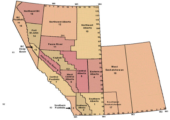
Source: petroCUBE
For an average well in each grouping, specific parameters were estimated, including: initial production rate, production decline curve conditions, average depth, gas composition, shrinkage, and success rate. Cost data obtained from petroCUBE, supplemented by publicly available information and consultations with industry, was calculated for the average well by region and formation. Additional details on the categories and cost inputs are given in Appendix 2.
For a gas well to be economic, total revenue from the production (less operating costs, royalties, taxes and a rate of return - ROR) has to offset the upfront costs (capital and land costs). Supply costs were calculated for wells without risk (assuming a well drilled will produce at the expected rate) and with risk (accounting for the chance that a well will be unsuccessful; that is, no hydrocarbons are found, the well is abandoned, and the land is reclaimed). The success rates are shown in Table 1.
For an average well in each grouping,[9] monthly cash flows were calculated over the producing lifetime of the well.[10] Cash flow represents the revenues[11] earned less expenses incurred over the life of each well. Expenses include capital, land, operating and processing, and reclamation costs. Royalties and taxes as they existed in 2009 were included. A 15 per cent rate of return to warrant investment was also included.[12]
[9] In this study, we used average numbers which aggregate the performance of thousands of wells. Every producing company is in a different position with respect to their own land holdings, cost structure, infrastructure, and experience.
[10] Production is assumed to stop in the first month that revenues are less than the ongoing expenses (operating and processing costs, royalties, and taxes).
[11] Revenues from natural gas (methane) as well as from NGLs (propane, butane, and pentanes plus).
[12] This 15 per cent after-tax rate translates into a higher ROR before tax.
The price level that generates sufficient revenue to offset the total expenses plus a return on investment establishes the supply cost for that resource grouping. This analysis is undertaken assuming that only successful wells were drilled (un-risked case), in addition to incorporating the costs of unsuccessful wells (risked case),[13] and sensitivities such as gas prices or capital cost changes. Additional details on the economic methodology used in the analysis are in Appendix 3.
[13] See Appendix A2.3.3.
Results
Supply Costs
Table 1 lists the supply costs and payout periods[14] for each resource grouping. The majority of gas production from wells drilled in 2009 came from resource groupings that have sufficient production history to model the decline curve parameters. In a few groupings, there was not enough data (either there were not enough producing wells or it was a new grouping) to determine the historical production profiles. For a few other groupings, the historical production data varied to such an extent that it did not provide a valid production decline curve. Groupings in both of these categories were evaluated with an estimated production decline curve, and are identified in Table 1 under ‘groupings with estimated decline curves'.
[14] Payout occurs when the cumulative sum of discounted cash flows, starting in the first period, equals zero.
Table 1: 2009 Supply Costs and Payouts for each Grouping
This table is available in Excel spreadsheet format [EXCEL 137 KB].
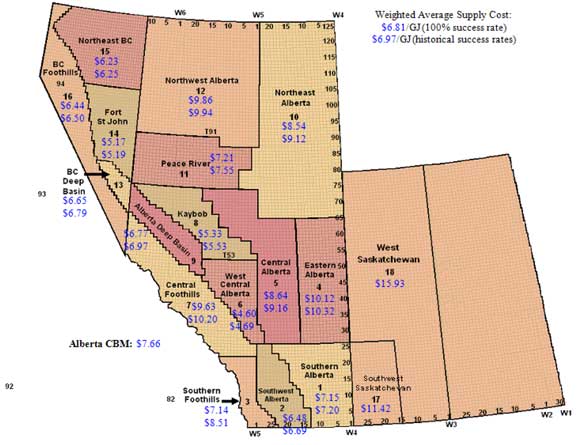
The weighted average[15] supply cost with a 100 per cent success rate (un-risked) for Western Canada was $6.81/GJ (Alberta Nova Inventory Transfer (NIT), Canadian dollars). Using 2009 success rates, the risked weighted average supply cost was $6.97/GJ. Success rates in Western Canada development wells are relatively high (weighted average of 96 per cent success in 2009) due to the advanced stage of development of many of these resources.[16] As a result, risked supply costs are generally not significantly higher than the un-risked versions. Figure 2 includes the risked and un-risked average supply costs for each area.
[15] Production in 2009 from 2009 drilled development wells by grouping is used to calculate the weighted averages.
[16] Exploration, test, disposal, and water wells are not included in the analysis since there is limited cost data available.
Given the $3.76/GJ average daily Alberta NIT price and an average supply cost of $6.97/GJ, on average, new gas development was uneconomic in 2009. However, some groupings did yield positive returns. These results are consistent with general impressions expressed by industry and are evident in the shift of gas activity away from conventional shallow gas sources towards the deep drilling of tight gas and shale gas plays in Alberta and British Columbia. The 2009 average supply cost for Alberta was $7.28/GJ, $5.96/GJ for B.C., and $12.87/GJ for Saskatchewan. In 2007, the B.C. and Alberta averages were almost equal at $7.81 and $7.84, respectively; Saskatchewan's average supply cost was $9.53. Saskatchewan experienced higher costs as increasing activity in Saskatchewan's Bakken and Shaunavon oil plays drove average land costs higher. The industry in Saskatchewan focuses on oil production and gas operations do not benefit from scale efficiencies.
The average natural gas supply cost in 2007 was $7.88/GJ, higher than the average market price of $6.11/GJ. The decrease in the average supply cost over the two years is mainly due to an increase in the average production rate per well, from an average initial production rate of 0.92 MMcf/d to 1.52 MMcf/d. This increased production rate overshadowed an increase in the capital cost of the average well, from $2.02 million/well in 2007 to $2.46 million/well in 2009. The increase in the average production rate and average capital cost in Western Canada was largely driven by Alberta tight gas development and Northeast B.C. plays in 2009, including the Montney tight gas and Horn River shale gas plays. Wells in these plays had high capital costs of more than $5 million/well but also had high producing rates, from 3.5 MMcf/d and up. The average supply cost for the Montney tight gas in the Fort St. John area was $3.92/GJ and the average supply cost for the Horn River shale gas in Northeast B.C. was $4.68/GJ.
Changes in operating and processing costs between 2007 and 2009 mostly cancelled each other out. The average operating costs decreased from $0.50/GJ in 2007 to $0.43/GJ in 2009 whereas the average processing costs increased from $0.52/GJ in 2007 to $0.62/GJ in 2009. The processing cost increases were driven by increased production from plays with high NGL content and associated processing costs, like the Montney play in the Fort St. John area. The lower operating costs were due, in part, to lower fuel and power costs. Drilling and service costs declined since 2007 as activity slowed and drillers were under pressure to cut service rates in an increasingly competitive market. Drilling efficiency improvements also reduced drilling costs. Other input costs, such as fuel, retreated from 2007 peaks, whereas material costs like casing and tubing costs, transportation and equipment rental costs increased since 2007. Overall, capital costs per well were higher because the average well in 2009 was deeper and more complex, as horizontal lengths were drilled from vertical holes.
Figure 2 : Average 2009 Supply Costs by Region
Price and Capital Cost Sensitivities
Sensitivity tests were performed on the six groupings with the highest new production totals in 2009. These top six groupings represent a wide variety of locations, including shallow and deep wells, and all four gas resource types.
To calculate supply cost sensitivities with gas price, the ROR is calculated for an assumed range of gas prices, from $3 to $12/GJ Alberta NIT. Figure 3 shows that at gas prices of $4/GJ, the deeper conventional, tight and shale groupings earn returns above zero whereas the shallow and CBM groupings need more than $6/GJ to earn positive returns. Gas price sensitivities for all groupings are in Appendix 12.
Figure 3: Rate of Return under various Gas Prices (un-risked)
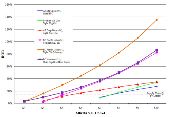
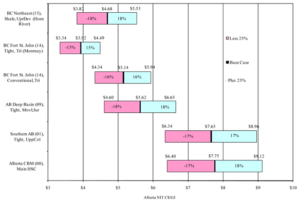
Figure 4 illustrates how supply costs change if total capital costs[17] increase or decrease by 25 per cent for the six groupings.[18] Some groupings were slightly more sensitive to capital cost changes than others. Supply costs change less than 25 per cent with a capital cost change of 25 per cent since there are other expenses including operating and processing costs, royalties, and taxes. For the most part, the supply cost changes were symmetrical for each grouping whether capital costs increased or decreased. Slight asymmetry arises depending on the capital deductions from royalties and taxes.
[17] Well drilling, tie-in, land, and reclamation costs.
[18] Note that the sensitivity examples are un-risked. This was done for ease of comparing capital costs - that is, to look at one drilling and completing capital cost instead of a weighted average of drilling and completing and drilling and abandonment capital costs and a lower expected production level than in Appendix 6, using probability of success. Note, however, that the risked and un-risked results would be equivalent for the CBM HSC region, the Fort St. John tight grouping and the Northeast B.C. shale grouping (100 per cent success rate), and very similar for the other regions (all success rates in the high 90s).
Figure 4: 2009 Supply Cost Capital Cost Sensitivities (un-risked)
Supply Cost Components
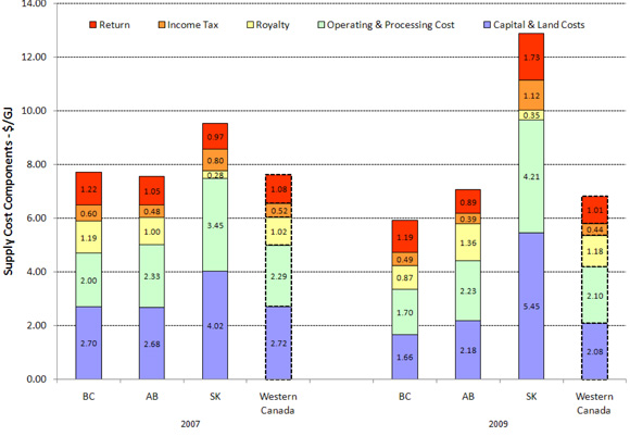
Figures 5 and 6 illustrate the components that make up the supply cost for each of the top six groupings, as well as the average for each province and for Western Canada. Capital and operating costs account for significant portions of all six groupings. Taxes and royalties vary provincially, as do capital cost allowances and other deductions. On average, Alberta groupings had a 19 per cent royalty rate and B.C. groupings had a 15 per cent royalty rate. The ROR portion depends on how long it takes before payout (see Table 1), that is, the longer it takes to pay back the capital investment, the more the return component is, as can be seen comparing the Montney to Horn River groupings. The CBM grouping had increased supply costs from 2007 to 2009, in part due to capital cost increases. However, the other shallow grouping in Southern Alberta had slightly lower capital costs, as activity in that area has continued to decline since 2007 and land prices have dropped. The deeper gas groupings had lower supply costs in 2009 compared to 2007, due to capital cost decreases and production rate increases. Appendix 13 includes a comparison of inputs and supply costs for 2007 and 2009. Appendix 14 lists the 2009 supply cost components for every grouping.
Figure 5: 2009 Supply Cost Components (un-risked)19
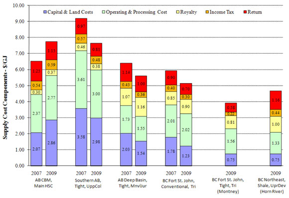
[19] There are no 2007 results for the Montney and Horn River groupings, as these groupings are relatively new, and data at that time was limited or did not exist.
Figure 6: Averaged Supply Cost Components (un-risked)
Observations
Natural gas drilling activity in Western Canada has remained low compared to the boom years of 2005 to 2008. The level of drilling activity is dependent on gas price and cost of production. This study illustrates the average cost structure in Western Canada and identifies the relative economics of various resource developments. There were positive economics for some areas and negative returns for others.
Looking forward, relatively lower gas prices will continue in 2010, however, supply costs of certain areas are expected to continue to decrease. Gas resources with higher NGL content have continued to see increased drilling activity into 2010, as oil prices remain high relative to natural gas prices. Increased knowledge of new resources, drilling efficiency improvements, decreasing costs per hydraulic fracture treatment, the ability to drill multiple wells from one well pad, and multi-lateral horizontal drilling have all led to supply cost decreases. Acquisitions will continue, especially in the deeper tight gas and shale gas developments in Canada and the U.S.A., as the larger producers benefit from economies of scale. Joint ventures have also benefited industry, as foreign investors have teamed up with Canadian and American shale gas producers to earn greater returns and gain knowledge.
Appendices
Appendix 1 - Cost Factors
Strong oil prices ($66.20/barrel at Edmonton averaged in 2009 or $10.82/GJ on an energy equivalency basis) meant producers involved in conventional and unconventional oil found it more attractive to invest in oil projects. Thus, budgets for natural gas activity were trimmed while the oil portion of budgets increased. This was evident from the increased share of rig activity for oil projects over gas projects in 2009. However, the oil pace could not outweigh the decline in gas activity, and weekly rig counts in 2009 dropped to an average of 233 in 2009, compared to 367 in 2007, lowering the drill-day and service-day costs.
Operating costs were lower in 2009 versus 2007 as the cost of fuel and power dropped by about 22 per cent on average[20] in Western Canada. Processing costs for new production in 2009 were higher as a result of increased production from plays with high NGL content that require additional processing, like the Montney play in the Fort St. John area.
[20] Petroleum Services Association of Canada. 2010 Well Cost Study, November 5, 2009.
Activity in oil plays and growth in oil sands increased other well costs in 2009 from 2007 levels. Casing, tubing, equipment rentals, and transportation costs increased on average.
Overall, the average capital cost of a well in Western Canada increased, from $2.02 million/well in 2007 to $2.46 million/well in 2009. The average well is deeper and more complex, such as in the large Northeast B.C. plays in 2009. This factor, along with the cost factors noted above, were the main drivers increasing average capital cost.
In addition, ongoing technology and efficiency improvements could lead to future declines in well costs.
Appendix 2 - Production and Cost Input Methodology
A2.1 Formation Groupings
For each region, the producing formations were grouped on a geological basis, and the supply costs were calculated for each of these groupings. The formations were grouped on the basis of similarities - depth and other physical attributes such as permeability and the type of resource (see Appendices 7 and 8), drilling costs and whether, in Alberta, the formations were allowed to be commingled.
A2.2 Resource Types
There were four resource types analyzed in this study - conventional gas, tight gas, coal bed methane (CBM) and shale. The split between conventional gas and tight gas is based on the tight gas plays defined by Forward Energy Group Inc.[21] Three main areas of tight gas recognized in this study include: certain Cretaceous zones in the Deep Basin; the Milk River, Medicine Hat and Second White Specks formations in southeast Alberta and southwest Saskatchewan; and the Jean Marie group in northeast B.C.
[21] Forward Energy Group Inc.
Newer developments for 2009 were not included in this analysis, as there was not enough data on the production profiles or cost estimates. Resource types excluded were tight gas in the Central Foothills Mannville grouping, tight gas in the lower Triassic and Mississippian groupings in Peace River, tight gas in the Mannville and Devonian groupings in Fort St. John, and other CBM areas besides the Horseshoe Canyon (HSC) and Mannville resources.
A2.3 Production Inputs
Historical well data[22] from 1998 to December 2009 was used to calculate the 2009 well inputs. The inputs were used to represent the average well in that grouping drilled in 2009. The inputs include initial production, production decline curve parameters, average depth, gas composition, shrinkage and success rate (probability that a well drilled will produce on average at the expected production level). Historical 2009 production was used as a basis for deriving the cost inputs for the groupings from the petroCUBE cost data (section A2.4).
[22] Well data from GeoScout
A2.3.1 Initial Production
Using 2009 well data, initial production rates for an average well in each grouping was determined by averaging initial rates for all wells.
A2.3.2 Decline Production Curve
For wells drilled[23] in each year (1998 to 2009), linear decline curves were fit, with decline rates and months at each decline rate modeled. For the earlier years, more data is available, and thus more complete decline curves can be modeled. For wells drilled in 2009, only their initial production rates and a few months of production were available, so historical curve analysis is used to extrapolate the performance of the 2009 wells. Initial production and decline parameter inputs are listed in Appendix 6.
[23] Wells that start producing in each year.
A2.3.3 Other Well Parameters
Historical data and previous NEB work is used to calculate average well depth, gas composition and shrinkage for each grouping. The resulting parameters can be found in Appendices 7 and 8.
To calculate the probability that a well drilled in a specific grouping will be successful (produce adequately), historical well data for each grouping was used. The ratio of successful versus unsuccessful wells was calculated for each grouping. For wells where the formation target was unknown but the depth known, statistical probability was used to estimate which formation was targeted. For each grouping, the well depth probability for each formation was modeled as a bell shaped normal distribution. If the well's depth was found to be within the formation's 80 per cent confidence range, that formation was identified as a possible target for the well. If there were more than one target formation found for a well, the formation in that area that had the most wells drilled was chosen as the target formation for that well. Also, normal distribution curves could not be modeled for formations that had few historical wells. In these cases, the eight surrounding townships' well data for that specific formation was pooled to estimate a normal distribution.
A2.4 Cost Inputs
Cost data from petroCUBE is available by region by formation (see Appendix 4 for a list of formations). The groupings used in this study sometimes contain more than one formation (see the ‘Resource Group' column in Appendix 5). Thus, historical well production data for 2009 is used to calculate ratios that were applied to the petroCUBE cost data. For each grouping, production data is summed for each formation. Ratios were calculated by formation (see Appendix 9), and these ratios were applied to the cost data to get average costs weighted by historical production. These costs were drilling and completion costs, tie-in costs, reclamation costs, land costs, processing costs and variable and fixed operating costs. Cost data was also gathered from public presentations, industry websites and industry consultations. See Appendices 10 and 11 for the cost input tables.
Appendix 3 - Economic Methodology
This appendix explains the details behind the cash flow analysis. Each grouping has cash flow determined using the assumptions described in this appendix and in Appendix 2. Cash flow sensitivities were examined by varying gas prices or capital costs. A total of 22 cash flow estimates were prepared for each grouping consisting of: one at today's costs and ten runs under varying gas price assumptions, all under a no risk assumption (probability of a successful well at 100 per cent) and a risked analysis (probability of a dry well, and its accompanying costs, taken into account). Twelve capital cost sensitivity tests were also run for six specific groupings.
A3.1 Cash Flow Analysis
Supply costs and ROR were calculated from the cash flow analysis. All cash flow components are in 2009 Canadian dollars. The net cash flow (NCF) for each time period is the total revenue less any costs and other payments due, such as taxes and royalties. The net cash flows for each time period were converted back to the first time period using a specified discount rate (the ROR) and summed to provide a net present value (NPV). The supply cost is the natural gas price that sets this NPV equal to zero. The supply cost can either be found for a specific ROR, or the ROR can be determined at a specified supply cost.
Payout can also be calculated after the supply cost or ROR is found. Payout occurs when the cumulative sum of discounted cash flows, starting in the first period, equals zero. Upfront capital costs lead to negative net cash flows in the first period, but as revenues are earned, the cumulative sum of cash flows will start to become positive, that is, as net earnings start to pay off the initial capital costs.
- Supply Cost and payout found given a 15 per cent ROR and NPV equal to zero
- ROR and payout found given a supply cost (sales price) and NPV equal to zero
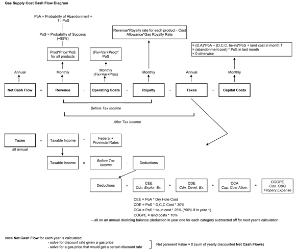
In this analysis production, costs and royalties were calculated on a monthly basis. The net monthly revenues, equal to production multiplied by price less costs and royalties, were summed together to get annual totals and then the taxable income and taxes due are calculated. The taxes due were subtracted from the net revenue to get annual net cash flows (NCF).
NCFy = Revenuey - Op. Costsy - Royalty Payabley - Taxes Payabley - Cap. Costsy
where
| Revenuei = | ∑ | Productionki * Pricekki |
| k |
Operating Costsi = Fixed Operating Costsi + Variable Operating Costsi
| Royalty Payablei = | ( | ∑ | Revenueki * Royalty Rateki) - Cost Allowancei * Royalty Ratei(gas) |
| k |
Taxes Payabley = Taxable Incomey * (Provincial Tax Ratey + Federal Tax Ratey)
| Capital Costsi | = Drilling, Casing, Completing, Tie-In costs + Land Costs in first month = Reclamation costs in last month of production = 0 otherwise |
i = month i
y = year y
k = product k (natural gas, propane, butane, pentanes plus and sulphur)
A3.2 Revenue
Revenue is determined by multiplying the marketable production volume by price, for each product. These revenues were summed to get total revenue. For some groupings, products other than natural gas were included. Butane, propane, pentanes plus and sulphur are all possible products of processing natural gas. Since these products produce income streams, this revenue needs to be accounted for in the well economics. The compositions of gas streams for each grouping are given in Appendix 7.
The natural gas price is either solved in the cash flow analysis as a supply cost, or it is assumed and inputted into the analysis to find the ROR. Prices tested range from $3 to $12/GJ, in one-dollar increments. The natural gas price is the market price per gigajoule in 2009 Canadian dollars. The price the producer receives at the wellhead is the market price less $0.15/GJ to account for transportation. This wellhead price is for 2009, and future prices were escalated at an annual real inflation rate of two per cent. For instance, if the price in 2009 is $3.85 (a market price of $4 less $0.15), the price in 2010 will be C2009$3.93/GJ (a two per cent real annual inflation applied to the $3.85), and so on for subsequent years of production.
Prices for the other products were assumed as follows. The plant gate sulphur price for 2009 is set at $37.29 per tonne, in 2009 Canadian dollars. It is then escalated for future years at a real annual inflation rate of two per cent.[24] Price ratios are applied to assign prices for the other products. The propane and butane prices for a given year were set at three times the wellhead natural gas price and the pentanes and heavier molecules (pentanes plus) price was set to four times the wellhead natural gas price. Converting raw gas into these different products required yield factors. The assumed factor for propane is 25.394 GJ per cubic metre of raw gas produced. The factor for butane is 28.345 GJ per cubic metre and 31.000 GJ per cubic metre for pentanes plus.
[24] The average annual inflation rate in Canada (using total Consumer Price Index (CPI)) was 1.6 per cent from 2007 to 2009.
A3.3 Success and Abandonment
Since there is a chance that a drilled well may be dry - unsuccessful for gas production - a probability is applied in the analysis to take this risk into account. The probability the well is unsuccessful and abandoned, for each grouping, is provided in Appendix 8. The probability of success - that the well drilled does produce adequately - is equal to one minus the probability of abandonment. To take this risk into account in the analysis, the production for each month is multiplied by the probability of success, to get an expected production, or risked production, and multiplied with costs each month.[25] Since revenue equals production multiplied by price, the revenue carried forward in all calculations is risked revenue, and along with the risked costs the economic analysis is an analysis including risk.
[25] Expected BTI = (Probability of Success)*BTI + (Probability of Abandonment)*zero BTI = (Probability of Success)*BTI since there is no income if the well is abandoned (dry).
A3.4 Capital Costs
Initial capital costs were assumed to apply in the first month of production, except for the reclamation cost, which occurs in the last month of production, and is escalated by the two per cent inflation rate. Note that unsuccessful wells have different capital costs (and no operating costs into the future since there is no production).
A3.5 Operating and Processing Costs
Operating costs are incurred every month of production. There are two types of operating costs - fixed and variable. Fixed operating costs are the same every month, regardless of how much is produced from the well that month. These could include equipment leases, maintenance and human resources. Variable operating costs, such as fuel and power, are a cost per unit of marketable production. The variable costs were in 2009 Canadian dollars and were the costs incurred in 2009. Future operating costs were inflated at the two per cent annual rate.
Raw gas needs to be processed into marketable gas before going to market. Processing costs are dollars per unit of production and are inflated at the two per cent real annual inflation rate.
A3.6 Royalties
Production is assumed to occur on Crown lands, which means royalties must be paid to the provincial government. Royalties exist because citizens own the natural resource (natural gas and natural gas liquids in this case) and must be compensated by producers who extract the resource for revenues.
Royalty frameworks in place as of December 2009 for British Columbia and Saskatchewan were used.[26] The new royalty framework for Alberta, released October 2007[27], was used in the Alberta economic analysis.[28] Gross royalties payable are the product of the royalty rate (in per cent) and the gross revenues (sales price assumed multiplied with production). Along with these gross royalty calculations, capital cost deductions, low productivity and deep well royalty relief adjustments were deducted from the gross royalty amounts to get actual net royalty amounts payable to the respective provincial government for each producing month.
[26] Oil and Gas Fiscal Regimes: Western Canadian Provinces and Territories, December 2006.
[27] Government of Alberta, About Royalties.
[28] The Alberta natural gas royalty formulas that are effective January 1, 2011 are not used, as they were not in existence until 2010.
A3.6.1 B.C. Royalties
The Base 9[29] gas royalty formula is used to calculate the B.C. gross royalties[30] for natural gas. This formula retains nine per cent of the price when the price is less than or equal to the select price, and 40 per cent of the price in excess of the select price. The assumed select price is $50/m³ ($1.41/Mcf). The royalty rate must be in the range of nine to 27 per cent. Wells producing less than 5000 10³m³/day on average for a month will see a decrease in the royalty rate.
[29] Gas produced from gas wells drilled on land acquired after June 1, 1998 which are completed within five years of the date rights are issued.
[30] For more information use the source noted in footnote 26 above.
Other products produced along with the natural gas were also subject to royalty payments. Royalties on natural gas liquids were levied at a flat rate of 20 per cent of the sales volume and royalties on sulphur were levied at a flat rate of 16 2/3 per cent of the sales volume. The gross royalty payable is the sum of all royalties payable for each product.
In B.C., producers can deduct cost allowances and qualifying deep well adjustments. Gas producers were eligible to receive the producer cost of service allowance (PCOS) for field gathering, dehydration, compression, field processing and conservation. That is, the total costs for these items, multiplied by the natural gas royalty rate, were deducted from gross royalties. Vertical wells that have a depth of at least 2500 metres or horizontal wells with a depth of 2300 metres qualify for deep well royalty holiday credits. This is applied to future royalties.[31]
[31] Since royalties payable cannot be negative, any amount of deductions exceeding the gross royalty payable for a month is carried forward into the next month and added to the deductions for that month, and so on until the deductions have all been used.
A3.6.2 Alberta Royalties
The royalty rate formulas for oil and gas in Alberta were updated in October 2007 with the provincial government's new royalty rate framework.[32] These new royalty formulas came into effect on January 1, 2009, and were used in this analysis.
[32] Government of Alberta, About Royalties.
The new natural gas royalty calculation is made up of two components - a price component and a quantity component. The sum of the two components makes up the royalty rate. Each component cannot exceed 30 per cent, and the sum - the total royalty rate - has a minimum of five per cent and a maximum of 50 per cent. The quantity component can also be decreased by a depth factor. If a well has a measured depth of 2000 metres or more, there will be a depth factor based on the quantity of gas produced. With this depth factor adjustment, the quantity component of the royalty rate can be negative. Royalty rates, as of December 2006, for propane, butane and methane were used in this analysis. The royalty rate is then multiplied by gross revenues to find the gross royalty in each month.
Like B.C., applicable costs can be deducted from the gross royalty, including annual capital costs, monthly operating costs and annual custom processing costs. These costs were multiplied by the natural gas royalty rate and subtracted from the total gross royalty amount to get a net royalty payable amount each month.
There is also a deep gas royalty relief in place. The Alberta government announced new deep resource programs to promote high cost oil and gas development on April 10, 2008. Those programs applied to wells that began drilling on or after April 10, 2008, and since this analysis is looking at the economics of 2009 drilled wells, these programs were included in the calculations.
A3.6.3 Saskatchewan Royalties
The royalty formula for ‘Fourth Tier[33] Gas from Gas Wells' is used to calculate the royalty rate for gas production in Saskatchewan. If the monthly gas production from a well is less than 25 10³m³/month, the royalty rate is zero per cent. If the monthly production is higher than 25 10³m³, the royalty rate is calculated based on one of two formulas - one if the production is higher than 115.4 10³m³/day and one if the production ranges from 25-115.4 10³m³/day.
[33] Gas produced from gas wells drilled on or after October 1, 2002.
There is also a cost allowance to reduce royalties payable, but unlike British Columbia and Alberta, the capital cost deduction is not based on dollars actually spent, but is a fixed gas cost allowance of $10 per thousand cubic metres for all gas types. This allowance is in recognition of the gathering and processing costs. There were no NGL royalties, so higher processing costs were not recognized in the allowance. Also, it is assumed that there is no sulphur production in Saskatchewan, and hence, no sulphur royalty.
A3.7 Taxes
New corporate tax rates in Canada were announced and passed in the fall of 2007, and were used in this analysis. The 2007 corporate income tax rate is 22.12 per cent for 2007, and will drop to 15 per cent by 2012. These rates presented below were used in the analysis and it is assumed that production beyond 2012 will face the 15 per cent tax rate.
| Canada Tax Rate | 2007 | 2008 | 2009 | 2010 | 2011 | 2012 |
|---|---|---|---|---|---|---|
| 22.12% | 19.5% | 19.0% | 18.0% | 16.5% | 15.0% |
Existing provincial tax rates, as of December 2009, were assumed. The provincial tax rates were assumed constant throughout the productive lifetime of each well. The tax rates were:
| Provincial Tax Rate | British Columbia | Alberta | Saskatchewan |
|---|---|---|---|
| 12% | 10% | 13% |
Before tax income (BTI) is revenue (production multiplied by price) less operating costs and royalty payable. BTI was calculated for each month and summed to provide a BTI for each calendar year. Taxable income is BTI less allowed depreciation and capital cost allowances in a given year. The tax rates were multiplied by the annual taxable income to get federal and provincial taxes payable for each producing year of a well. Annual after tax income (ATI) is then calculated by subtracting the taxes payable from the BTI for each year.
A3.8 Net Cash Flows (NCF) and Solving
The NCF for each year is the risked ATI less capital costs. The initial capital costs are assumed to occur in the first month, so the net cash flow in the first month will be negative. The reclamation cost in the last producing month will also lead to negative cash flow for that month in most cases. For all other months, there are no assumed capital costs, and since production will only continue while the revenues can cover the operating costs, net cash flows are positive. As production falls, the revenue will, at some point, not cover operating costs and hence, production is assumed to stop.
The costs must also be weighed by the probability of success. If the well is abandoned, the producer will incur land, drilling and abandonment costs and a reclamation cost. If the well is successful, the producer will incur land costs, drilling, casing and tie-in costs and reclamation costs. So, the total initial capital cost is:
| Initial Capital Cost = | land costs + (probability of an unsuccessful well) * dry hole cost + (probability of success)* (drilling, casing costs + tie-in costs) |
The capital cost in the last production month is the inflated reclamation cost. Once the NCF's were determined, the NPV and payouts were calculated, as well as either the ROR or the supply cost for an average well in each grouping.
A summary of the economic methodology is presented in Figure A1.
Figure A1: Cash Flow Diagram
Appendix 4 - Formations
| Abbreviation | Resource Group |
|---|---|
| Tert | Tertiary |
| UprCret | Upper Cretaceous |
| UprCol | Upper Colorado |
| Colr | Colorado |
| UprMnvl | Upper Mannville |
| MdlMnvl | Middle Mannville |
| LwrMnvl | Lower Mannville |
| Mnvl | Mannville |
| Jur | Jurassic |
| UprTri | Upper Triassic |
| LwrTri | Lower Triassic |
| Tri | Triassic |
| Perm | Permian |
| Miss | Mississippian |
| UprDvn | Upper Devonian |
| MdlDvn | Middle Devonian |
| LwrDvn | Lower Devonian |
Note, for example, the Mannville formation is listed as Mnvl, or could be split up into the upper, middle and lower Mannville formations.
Appendix 5 - Groupings
| Area Name | Area Number | Resource Type | Resource Group |
|---|---|---|---|
| CBM Area CBM Area |
00 00 |
CBM CBM |
Main HSC Mannville |
| Southern Alberta Southern Alberta Southern Alberta Southern Alberta |
01 01 01 01 |
Conventional Conventional Conventional Tight |
Tert;UprCret;UprColr Colr Mnvl UprColr |
| Southwest Alberta Southwest Alberta Southwest Alberta Southwest Alberta Southwest Alberta Southwest Alberta Southwest Alberta |
02 02 02 02 02 02 02 |
Conventional Conventional Conventional Conventional Tight Tight Tight |
Tert;UprCret;UprColr Colr MdlMnvl;LwrMnvl Jur;Miss UprColr Colr LwrMnvl |
| Southern Foothills | 03 | Conventional | Miss;UprDvn |
| Eastern Alberta Eastern Alberta Eastern Alberta |
04 04 04 |
Conventional Conventional Tight |
UprCret;UprColr Colr;Mnvl UprColr |
| Central Alberta Central Alberta Central Alberta Central Alberta Central Alberta Central Alberta |
05 05 05 05 05 05 |
Conventional Conventional Conventional Conventional Tight Tight |
Tert;UprCret Colr Mnvl Miss;UprDvn Colr Mnvl |
| West Central Alberta West Central Alberta West Central Alberta West Central Alberta West Central Alberta West Central Alberta West Central Alberta West Central Alberta |
06 06 06 06 06 06 06 06 |
Conventional Conventional Conventional Conventional Conventional Conventional Tight Tight |
Tert UprCret;UprColr Mnvl LwrMnvl; Jur Miss UprDvn Colr Mnvl |
| Central Foothills Central Foothills Central Foothills Central Foothills Central Foothills Central Foothills Central Foothills |
07 07 07 07 07 07 07 |
Conventional Conventional Conventional Conventional Conventional Tight Tight |
UprColr Colr;Mnvl Jur;Tri;Perm Miss UprDvn;MdlDvn UprColr;Colr Jur |
| Kaybob Kaybob Kaybob Kaybob Kaybob |
08 08 08 08 08 |
Conventional Conventional Conventional Conventional Tight |
UprColr;Colr Mnvl;Jur Tri UprDvn Colr;Mnvl |
| Alberta Deep Basin Alberta Deep Basin Alberta Deep Basin Alberta Deep Basin Alberta Deep Basin Alberta Deep Basin Alberta Deep Basin Alberta Deep Basin |
09 09 09 09 09 09 09 09 |
Conventional Conventional Conventional Conventional Conventional Tight Tight Tight |
UprCret UprColr Mnvl;Jur Tri UprDvn UprColr Colr Mnvl;Jur |
| Northeast Alberta | 10 | Conventional | Mnvl;UprDvn |
| Peace River Peace River Peace River Peace River Peace River Peace River Peace River Peace River Peace River |
11 11 11 11 11 11 11 11 11 |
Conventional Conventional Conventional Conventional Conventional Conventional Conventional Tight Tight |
UprColr Colr;UprMnvl MdlMnvl;LwrMnvl UprTri LwrTri Miss UprDvn;MdlDvn UprColr MdlMnvl;LwrMnvl |
| Northwest Alberta Northwest Alberta Northwest Alberta Northwest Alberta |
12 12 12 12 |
Conventional Conventional Conventional Conventional |
Mnvl Miss UprDvn MdlDvn |
| BC Deep Basin BC Deep Basin BC Deep Basin BC Deep Basin BC Deep Basin |
13 13 13 13 13 |
Conventional Conventional Tight Tight Tight |
Colr LwrTri Colr Mnvl LwrTri |
| Fort St. John Fort St. John Fort St. John Fort St. John Fort St. John Fort St. John |
14 14 14 14 14 14 |
Conventional Conventional Conventional Conventional Tight Tight |
Mnvl Tri Perm;Miss UprDvn;MdlDvn Tri Perm;Miss |
| Northeast BC Northeast BC Northeast BC Northeast BC Northeast BC |
15 15 15 15 15 |
Conventional Conventional Conventional Tight Shale |
LwrMnvl Perm;Miss UprDvn;MdlDvn UprDvn MdlDvn |
| BC Foothills BC Foothills |
16 16 |
Conventional Conventional |
Colr;Mnvl Tri;Perm;Miss |
| Southwest Saskatchewan | 17 | Tight | UprColr |
| West Saskatchewan West Saskatchewan |
18 18 |
Conventional Conventional |
Colr MdlMnvl;LwrMnvl;Miss |
Appendix 6 - Decline Parameters
This appendix is available in Excel spreadsheet format [EXCEL 133 KB].
Appendix 7 - Gas Compositions
| Area | RsrcType | Resource Group |
Resource Group |
C3 barrels per marketable mmcf |
C4 barrels marketable mmcf |
C5+ barrels marketable mmcf |
Sulphur tonnes per marketable mmcf |
|---|---|---|---|---|---|---|---|
| 00 00 |
CBM CBM |
Main HSC Mannville |
Main HSC Mannville |
0 0 |
0 0 |
0 0 |
0 0 |
| 01 01 01 01 |
Conventional Conventional Conventional Tight |
02;03;04 05 06;07;08 04 |
Tert;UprCret;UprColr Colr Mnvl UprColr |
0 0.05 0.38 0 |
0.08 0.48 1.67 0.1 |
0.41 1.92 5.21 0.39 |
0 0.0007 0.0025 0 |
| 02 02 02 02 02 02 02 |
Conventional Conventional Conventional Conventional Tight Tight Tight |
02;03;04 05 06;07;08 09;13 04 05 08 |
Tert;UprCret;UprColr Colr MdlMnvl;LwrMnvl Jur;Miss UprColr Colr Lwr Mnvl |
0.02 0 0.46 0.75 0 0.1 0.6 |
0.12 0.2 1.91 2.69 0.04 0.63 2.07 |
0.44 0.94 7.01 13.11 0.23 1.8 8.22 |
0.001 0.0009 0.0109 0.1813 0 0 0.0829 |
| 03 | Conventional | 13;14 | Miss;UprDvn | 5.94 | 6.04 | 21.6 | 4.2071 |
| 04 04 04 |
Conventional Conventional Tight |
03;04 05;06;07;08 04 |
UprCret;UprColr Colr;Mnvl UprColr |
0 0.02 0 |
0.06 0.28 0.03 |
0.28 0.96 0.13 |
0.0008 0.0017 0 |
| 05 05 05 05 05 05 |
Conventional Conventional Conventional Conventional Tight Tight |
02;03 05 06;07;08 13;14 05 06;07;08 |
Tert;UprCret Colr Mnvl Miss;UprDvn Colr Mnvl |
0.01 0.31 0.65 1.21 0.57 0.94 |
0.16 0.95 1.86 3.64 2.15 3.39 |
0.72 3.17 5.12 12.31 7.96 10.77 |
0.0016 0 0.0101 0.2296 0.0114 0.0095 |
| 06 06 06 06 06 06 06 06 |
Conventional Conventional Conventional Conventional Conventional Conventional Tight Tight |
02 03;04 06;07;08 08;09 13 14 05 06;07;08 |
Tert UprCret;UprColr Mnvl LwrMnvl;Jur Miss UprDvn Colr Mnvl |
0.06 6.92 6.36 6.21 3.39 18.8 4.46 7.87 |
0.38 6.23 5.77 5.63 4.06 23.36 4.76 6.61 |
1.67 20.48 15.04 16.55 16.75 94.98 14.58 16.64 |
0.0043 0.0153 0.0034 0.0218 0.2376 4.6315 0.0226 0.0939 |
| 07 07 07 07 07 07 07 |
Conventional Conventional Conventional Conventional Conventional Tight Tight |
04 05;06;07;08 09;10;11;12 13 14;15 04;05 09 |
UprColr Colr;Mnvl Jur;Tri;Perm Miss UprDvn;MdlDvn UprColr;Colr Jur |
7.08 0.9 0.07 1.23 0.06 0.73 0 |
4.86 1.34 0.21 1.2 0.28 2.66 0.19 |
14.08 4.73 1.12 3.68 2.35 18.78 1.35 |
0.0963 0.0909 0.9984 1.6192 4.2066 0.3842 0 |
| 08 08 08 08 08 |
Conventional Conventional Conventional Conventional Tight |
04;05 06;07;08;09 10;11 14 05;06;07;08 |
UprColr;Colr Mnvl;Jur Tri UprDvn Colr;Mnvl |
5.16 2.3 10.37 17.48 11.11 |
3.89 2.91 7.48 18.04 6.69 |
7.84 8.88 18.88 81.7 11.5 |
0.0023 0.0199 0.7438 3.1326 0.0259 |
| 09 09 09 09 09 09 09 09 |
Conventional Conventional Conventional Conventional Conventional Tight Tight Tight |
03 04 06;07;08;09 10;11 14 04 05 06;07;08;09 |
UprCret UprColr Mnvl;Jur Tri UprDvn UprColr Colr Mnvl;Jur |
3.56 11.71 8.36 3.53 0.53 5.67 6.98 8.63 |
3.68 6.89 5.05 2.06 1.18 5.1 3.96 4.64 |
8.18 12.63 9.82 5.49 10.56 15 9.45 8.79 |
0 0.0041 0.0559 1.2427 4.7413 0.013 0.1195 0.0167 |
| 10 | Conventional | 06;07;08;14 | Mnvl;UprDvn | 0 | 0.01 | 0.04 | 0 |
| 11 11 11 11 11 11 11 11 11 |
Conventional Conventional Conventional Conventional Conventional Conventional Conventional Tight Tight |
04 05;06 07;08 10 11 13 14;15 04 07;08 |
UprColr Colr;UprMnvl MdlMnvl;LwrMnvl UprTri LwrTri Miss UprDvn;MdlDvn UprColr MdlMnvl;LwrMnvl |
0.31 0.43 0.16 0.86 0.74 5.67 0.42 0.31 0 |
0.69 0.29 0.45 1.5 2.19 4.43 2.15 0.69 0.26 |
2.52 1.87 2.96 4.95 9.33 11.9 5.96 2.52 1.07 |
0.0013 0.002 0.0045 0.21 0.4875 0.0056 0.097 0.0013 0 |
| 12 12 12 12 |
Conventional Conventional Conventional Conventional |
06;07;08 13 14 15 |
Mnvl Miss UprDvn MdlDvn |
0.09 0 0.53 4.77 |
0.44 0.16 2.55 3.48 |
1.39 0.56 14.59 7.51 |
0.0008 0 0.0644 0.5341 |
| 13 13 13 13 13 |
Conventional Conventional Tight Tight Tight |
05 11 05 06;07;08 11 |
Colr LwrTri Colr Mnvl LwrTri |
2.65 0.42 0 0.09 0.13 |
2.31 0.35 0.26 0.18 0 |
3.44 0.41 1.07 0.61 0 |
0 0.2479 0 0 28 |
| 14 14 14 14 14 14 |
Conventional Conventional Conventional Conventional Tight Tight |
06;07;08 10;11 12; 13 14;15 11 12;13 |
Mnvl Tri Perm;Miss UprDvn;MdlDvn Tri Perm;Miss |
15.96 10.71 3.26 0.03 8.05 3.26 |
8.14 6.91 2.97 0.06 4.12 2.97 |
7.19 7.63 6.45 4 6.88 6.45 |
0.0242 0.5024 0.0818 0.0402 0 0.0818 |
| 15 15 15 15 15 |
Conventional Conventional Conventional Tight Shale |
08 12;13 14;15 14 14 |
LwrMnvl Perm;Miss UprDvn;MdlDvn UprDvn Shale |
8.27 0.03 0.13 0 0 |
6.74 0.08 0.15 0.15 0 |
8.05 0.31 0.18 1.47 0 |
0 0.0467 0.5967 0.0027 0 |
| 16 16 |
Conventional Conventional |
05;06;07;08 10;11;12;13 |
Colr;Mnvl Tri;Perm;Miss |
0.64 0.01 |
0.59 0.06 |
0.67 0.24 |
0.005 2.9532 |
| 17 | Tight | 04 | UprColr | 0 | 0.1 | 0.39 | 0 |
| 18 18 |
Conventional Conventional |
05 07;08;13 |
Colr MdlMnvl;LwrMnvl;Miss |
0.02 0.02 |
0.28 0.28 |
0.96 0.96 |
0.0017 0.0017 |
Appendix 8 - Other Well Parameters
| Area | Resource Type |
Resource Group |
Total Measured Depth m |
Shrinkage % after processing |
Probability of Success % |
|---|---|---|---|---|---|
| 00 00 |
CBM CBM |
Main HSC Mannville |
760 2081 |
95.0% 95.0% |
100.0% 100.0% |
| 01 01 01 01 |
Conventional Conventional Conventional Tight |
Tert;UprCret;UprColr Colr Mnvl UprColr |
809 760 1167 693 |
95.5% 95.0% 92.2% 94.4% |
99.9% 93.5% 90.0% 99.6% |
| 02 02 02 02 02 02 02 |
Conventional Conventional Conventional Conventional Tight Tight Tight |
Tert;UprCret;UprColr Colr MdlMnvl;LwrMnvl Jur;Miss UprColr Colr LwrMnvl |
962 1308 1765 2236 390 2403 2460 |
94.0% 94.5% 88.3% 86.6% 95.4% 94.8% 90.9% |
95.5% 62.5% 97.0% 100.0% 99.9% 65.0% 99.9% |
| 03 | Conventional | Miss;UprDvn | 3900 | 63.5% | 80.0% |
| 04 04 04 |
Conventional Conventional Tight |
UprCret;UprColr Colr;Mnvl UprColr |
479 836 896 |
95.4% 94.7% 95.8% |
96.0% 95.0% 90.0% |
| 05 05 05 05 05 05 |
Conventional Conventional Conventional Conventional Tight Tight |
Tert;UprCret Colr Mnvl Miss;UprDvn Colr Mnvl |
922 1343 1158 1673 1524 1867 |
93.5% 94.4% 91.9% 89.1% 92.1% 90.2% |
99.0% 98.0% 78.0% 93.0% 99.9% 92.3% |
| 06 06 06 06 06 06 06 06 |
Conventional Conventional Conventional Conventional Conventional Conventional Tight Tight |
Tert UprCret;UprColr Mnvl LwrMnvl;Jur Miss UprDvn Colr Mnvl |
1199 1666 2810 2775 2732 3529 1742 2856 |
90.9% 87.2% 86.7% 84.8% 84.5% 51.5% 88.7% 84.4% |
97.0% 91.0% 100.0% 93.0% 95.0% 75.0% 91.7% 95.3% |
| 07 07 07 07 07 07 07 |
Conventional Conventional Conventional Conventional Conventional Tight Tight |
UprColr Colr;Mnvl Jur;Tri;Perm Miss UprDvn;MdlDvn UprColr;Colr Jur |
3546 3588 3399 3580 3897 2955 4640 |
88.5% 91.1% 87.4% 81.8% 69.3% 87.9% 95.7% |
75.0% 97.0% 99.0% 81.0% 100.0% 100.0% 100.0% |
| 08 08 08 08 08 |
Conventional Conventional Conventional Conventional Tight |
UprColr;Colr Mnvl;Jur Tri UprDvn Colr;Mnvl |
2463 2709 3363 3828 3044 |
90.5% 89.7% 82.2% 64.4% 84.9% |
66.7% 91.7% 94.7% 93.0% 92.9% |
| 09 09 09 09 09 09 09 09 |
Conventional Conventional Conventional Conventional Conventional Tight Tight Tight |
UprCret UprColr Mnvl;Jur Tri UprDvn UprColr Colr Mnvl;Jur |
1090 2886 3068 3623 4529 2463 3096 3182 |
91.2% 86.2% 84.6% 84.1% 70.1% 88.7% 85.6% 85.3% |
92.0% 97.8% 100.0% 100.0% 75.0% 97.8% 92.0% 94.1% |
| 10 | Conventional | Mnvl;UprDvn | 520 | 95.1% | 81.1% |
| 11 11 11 11 11 11 11 11 11 |
Conventional Conventional Conventional Conventional Conventional Conventional Conventional Tight Tight |
UprColr Colr;UprMnvl MdlMnvl;LwrMnvl UprTri LwrTri Miss UprDvn;MdlDvn UprColr MdlMnvl;LwrMnvl |
634 872 1590 1070 2650 1805 2395 695 1390 |
94.5% 94.6% 92.4% 90.5% 88.7% 88.8% 89.0% 94.5% 92.4% |
76.0% 80.0% 78.8% 96.0% 99.0% 100.0% 62.5% 95.0% 95.0% |
| 12 12 12 12 |
Conventional Conventional Conventional Conventional |
Mnvl Miss UprDvn MdlDvn |
982 486 1957 1531 |
94.1% 90.7% 90.8% 84.0% |
100.0% 100.0% 87.5% 100.0% |
| 13 13 13 13 13 |
Conventional Conventional Tight Tight Tight |
Colr LwrTri Colr Mnvl LwrTri |
3216 4452 3216 3850 4055 |
95.1% 91.7% 96.4% 95.2% 95.0% |
50.0% 98.3% 100.0% 99.3% 100.0% |
| 14 14 14 14 14 14 |
Conventional Conventional Conventional Conventional Tight Tight |
Mnvl Tri Perm;Miss UprDvn;MdlDvn Tri Perm;Miss |
1062 2086 3143 4055 4055 4055 |
85.2% 85.2% 91.9% 89.3% 95.0% 95.2% |
98.0% 99.1% 100.0% 100.0% 100.0% 100.0% |
| 15 15 15 15 15 |
Conventional Conventional Conventional Tight Shale |
LwrMnvl Perm;Miss UprDvn;MdlDvn UprDvn Shale |
1219 762 1962 2558 4460 |
92.6% 89.4% 79.7% 95.3% 85.0% |
100.0% 100.0% 95.0% 98.1% 100.0% |
| 16 16 |
Conventional Conventional |
Colr;Mnvl Tri;Perm;Miss |
2990 2741 |
90.9% 78.3% |
98.4% 99.0% |
| 17 | Tight | UprColr | 583 | 86.0% | 100.0% |
| 18 18 |
Conventional Conventional |
Colr MdlMnvl;LwrMnvl;Miss |
740 852 |
80.0% 80.0% |
100.0% 100.0% |
Appendix 9 - Formation Ratios by Grouping
This appendix is available in Excel spreadsheet format [EXCEL 139 KB].
Appendix 10 - 2009 Capital Costs
| Area | Resource Type |
Resource Group |
Drill & Abandon Cost (unsuccessful well) Thousands C$ |
Drill & Comp Cost (successful well) Thousands C$ |
Tie-In Costs Thousands C$ |
Reclamation Costs Thousands C$ |
Land Costs C$ |
|---|---|---|---|---|---|---|---|
| 00 00 |
CBM CBM |
Main HSC Mannville |
126 504 |
310 1239 |
60 60 |
70 70 |
40 40 |
| 01 01 01 01 |
Conventional Conventional Conventional Tight |
02;03;04 05 06;07;08 04 |
106 212 305 126 |
185 400 511 208 |
50 124 131 50 |
35 48 63 35 |
4 4 4 4 |
| 02 02 02 02 02 02 02 |
Conventional Conventional Conventional Conventional Tight Tight Tight |
02;03;04 05 07;08 09;13 04 05 08 |
130 278 450 485 160 292 438 |
236 480 678 735 270 504 668 |
50 50 50 50 50 50 50 |
70 70 70 70 70 70 70 |
14 14 14 14 14 14 14 |
| 03 | Conventional | 13;14 | 12135 | 15815 | 2000 | 74 | 128 |
| 04 04 04 |
Conventional Conventional Tight |
03;04 05;06;07;08 04 |
178 222 185 |
343 418 352 |
114 113 113 |
41 51 40 |
13 12 12 |
| 05 05 05 05 05 05 |
Conventional Conventional Conventional Conventional Tight Tight |
02;03 05 06;07;08 13;14 05 06;07;08 |
133 212 286 522 215 286 |
323 435 558 837 439 557 |
106 106 106 106 106 106 |
45 68 70 70 69 70 |
14 14 14 14 14 14 |
| 06 06 06 06 06 06 06 06 |
Conventional Conventional Conventional Conventional Conventional Conventional Tight Tight |
02 03;04 06;07;08 08;09 13 14 05 06;07;08 |
136 170 304 350 448 494 263 314 |
250 325 714 974 1300 1431 639 729 |
72 72 195 214 184 180 72 195 |
45 74 75 75 75 75 75 75 |
60 60 60 60 60 60 60 60 |
| 07 07 07 07 07 07 07 |
Conventional Conventional Conventional Conventional Conventional Tight Tight |
04 05;06;07;08 09;10;11;12 13 14;15 04;05 09 |
1620 2238 4015 5364 6077 2016 3262 |
3330 4015 6069 7743 8712 3769 5154 |
1500 1500 1500 1500 1500 1500 1500 |
85 85 85 85 85 85 85 |
570 570 570 570 570 570 570 |
| 08 08 08 08 08 |
Conventional Conventional Conventional Conventional Tight |
04;05 06;07;08;09 10;11 14 05;06;07;08 |
484 660 861 1052 594 |
897 1092 1316 1529 1020 |
180 179 180 180 180 |
75 75 75 75 75 |
171 170 171 171 171 |
| 09 09 09 09 09 09 09 09 |
Conventional Conventional Conventional Conventional Conventional Tight Tight Tight |
03 04 06;07;08;09 10;11 14 04 05 06;07;08;09 |
1054 1281 1752 2184 4531 1426 1356 1688 |
1755 1994 2552 3751 6325 2328 2244 2611 |
270 270 270 270 269 270 270 270 |
80 80 80 80 80 80 80 80 |
81 81 81 81 81 81 81 81 |
| 10 | Conventional | 06;07;08;14 | 199 | 380 | 150 | 53 | 14 |
| 11 11 11 11 11 11 11 11 11 |
Conventional Conventional Conventional Conventional Conventional Conventional Conventional Tight Tight |
04 05;06 07;08 10 11 13 14;15 UprColr MdlMnvl;LwrMnvl |
515 657 1005 1174 1459 1013 1700 525 1050 |
954 1102 1465 1683 2006 1545 2332 972 1526 |
270 270 270 270 270 270 270 270 270 |
55 71 75 75 75 75 75 55 75 |
99 99 99 99 99 99 99 99 99 |
| 12 12 12 12 |
Conventional Conventional Conventional Conventional |
06;07;08 13 14 15 |
206 273 537 999 |
631 676 931 1424 |
414 414 414 414 |
56 55 89 94 |
112 112 112 112 |
| 13 13 13 13 13 |
Conventional Conventional Tight Tight Tight |
05 11 05 06;07;08 11 |
1195 1665 1195 1558 1665 |
2125 2650 2125 2531 5550 |
300 300 300 300 300 |
80 80 80 80 80 |
2345 2345 2345 2345 2345 |
| 14 14 14 14 14 14 |
Conventional Conventional Conventional Conventional Tight Tight |
06;07;08 10;11 12;13 14;15 Tri Perm;Miss |
762 1010 1348 2314 935 1317 |
1355 1733 2010 3139 5550 5950 |
285 430 430 430 430 430 |
100 100 100 100 100 100 |
261 261 261 261 261 261 |
| 15 15 15 15 15 |
Conventional Conventional Conventional Tight Shale |
08 12;13 14;15 14 Shale |
935 787 3358 2849 3223 |
1480 1315 4275 3630 6424 |
413 413 415 415 415 |
75 65 75 75 75 |
1970 1970 1970 1970 1970 |
| 16 16 |
Conventional Conventional |
05;06;07;08 10;11;12;13 |
2900 3489 |
4623 5278 |
300 354 |
85 85 |
927 927 |
| 17 | Tight | 04 | 100 | 161 | 40 | 35 | 145 |
| 18 18 |
Conventional Conventional |
05 07;08;13 |
185 257 |
385 465 |
109 | 64 | 144 |
Appendix 11 - 2009 Operating and Processing Costs
| Area | Resource Type |
Resource Group |
Variable Operating Cost | Fixed Operating Cost | Processing Cost | ||
|---|---|---|---|---|---|---|---|
| $/10³m³ | $/mcf | $/month | $/10³m³ | $/mcf | |||
| 00 00 |
CBM CBM |
Main HSC Mannville |
17.75 17.75 |
0.50 0.50 |
1000 1000 |
21.30 21.30 |
0.60 0.60 |
| 01 01 01 01 |
Conventional Conventional Conventional Tight |
Tert;UprCret;UprColr Colr Mnvl UprColr |
8.21 8.53 8.53 8.33 |
0.23 0.24 0.24 0.23 |
775.00 927.79 976.71 775.00 |
28.39 28.39 33.19 28.39 |
0.80 0.80 0.94 0.80 |
| 02 02 02 02 02 02 02 |
Conventional Conventional Conventional Conventional Tight Tight Tight |
Tert;UprCret;UprColr Colr MdlMnvl;LwrMnvl Jur;Miss UprColr Colr LwrMnvl |
8.82 8.82 9.10 10.61 8.82 8.82 9.11 |
0.25 0.25 0.26 0.30 0.25 0.25 0.26 |
1050.00 1050.00 1169.27 1488.11 1050.00 1050.94 1174.70 |
40.82 40.82 44.20 46.63 40.82 40.84 44.36 |
1.15 1.15 1.25 1.31 1.15 1.15 1.25 |
| 03 | Conventional | Miss;UprDvn | 24.02 | 0.68 | 15608.35 | 42.29 | 1.19 |
| 04 04 04 |
Conventional Conventional Tight |
UprCret;UprColr Colr;Mnvl UprColr |
9.79 9.40 9.33 |
0.28 0.26 0.26 |
1458.60 1655.21 1500.00 |
35.23 32.62 24.85 |
0.99 0.92 0.70 |
| 05 05 05 05 05 05 |
Conventional Conventional Conventional Conventional Tight Tight |
Tert;UprCret Colr Mnvl Miss;UprDvn Colr Mnvl |
8.87 8.87 8.87 8.87 8.87 10.65 |
0.25 0.25 0.25 0.25 0.25 0.30 |
1987.13 2260.80 2677.18 2700.00 1513.68 1780.83 |
24.85 25.56 28.11 34.02 28.39 32.65 |
0.70 0.72 0.79 0.96 0.80 0.92 |
| 06 06 06 06 06 06 06 06 |
Conventional Conventional Conventional Conventional Conventional Conventional Tight Tight |
Tert UprCret;UprColr Mnvl LwrMnvl;Jur Miss UprDvn Colr Mnvl |
8.13 11.18 16.19 16.19 17.16 17.26 11.23 16.24 |
0.23 0.31 0.46 0.46 0.48 0.49 0.32 0.46 |
1450.00 3023.25 3076.63 3303.56 3882.48 4015.78 3050.00 3098.99 |
24.85 25.56 26.98 28.39 35.49 39.84 25.56 26.98 |
0.70 0.72 0.76 0.80 1.00 1.12 0.72 0.76 |
| 07 07 07 07 07 07 07 |
Conventional Conventional Conventional Conventional Conventional Tight Tight |
UprColr Colr;Mnvl Jur;Tri;Perm Miss UprDvn;MdlDvn UprColr;Colr Jur |
34.39 34.28 34.28 34.28 34.28 34.39 34.11 |
0.97 0.97 0.97 0.97 0.97 0.97 0.96 |
9250.00 9250.00 9250.00 9250.00 9250.00 9250.00 9250.00 |
28.84 23.07 28.23 30.12 31.97 26.53 23.96 |
0.81 0.65 0.80 0.85 0.90 0.75 0.68 |
| 08 08 08 08 08 |
Conventional Conventional Conventional Conventional Tight |
UprColr;Colr Mnvl;Jur Tri UprDvn Colr;Mnvl |
16.14 20.83 21.00 27.11 20.95 |
0.45 0.59 0.59 0.76 0.59 |
3318.83 3747.86 3890.68 3924.53 3629.14 |
19.49 27.17 31.15 42.59 25.79 |
0.55 0.77 0.88 1.20 0.73 |
| 09 09 09 09 09 09 09 09 |
Conventional Conventional Conventional Conventional Conventional Tight Tight Tight |
UprCret UprColr Mnvl;Jur Tri UprDvn UprColr Colr Mnvl;Jur |
19.17 19.17 18.73 18.76 22.42 19.17 19.17 21.12 |
0.54 0.54 0.53 0.53 0.63 0.54 0.54 0.59 |
3960.00 3960.04 3612.30 3949.03 6502.57 3960.00 3960.00 3583.83 |
10.65 10.65 12.89 15.52 22.97 10.65 10.65 10.94 |
0.30 0.30 0.36 0.44 0.65 0.30 0.30 0.31 |
| 10 | Conventional | Mnvl;UprDvn | 7.68 | 0.22 | 2692.26 | 18.88 | 0.53 |
| 11 11 11 11 11 11 11 11 11 |
Conventional Conventional Conventional Conventional Conventional Conventional Conventional Tight Tight |
UprColr Colr;UprMnvl MdlMnvl;LwrMnvl UprTri LwrTri Miss UprDvn;MdlDvn UprColr MdlMnvl;LwrMnvl |
10.65 10.65 7.81 7.81 7.81 7.81 8.87 10.65 10.65 |
0.30 0.30 0.22 0.22 0.22 0.22 0.25 0.30 0.30 |
4000.00 4032.82 5000.00 5000.00 4500.00 5000.00 6000.00 4000.00 4050.00 |
17.75 17.75 17.75 25.12 26.42 22.99 23.04 17.75 17.75 |
0.50 0.50 0.50 0.71 0.74 0.65 0.65 0.50 0.50 |
| 12 12 12 12 |
Conventional Conventional Conventional Conventional |
Mnvl Miss UprDvn MdlDvn |
8.56 12.05 12.43 11.28 |
0.24 0.34 0.35 0.32 |
4439.71 5151.16 5514.04 6053.42 |
17.78 27.39 36.44 39.74 |
0.50 0.77 1.03 1.12 |
| 13 13 13 13 13 |
Conventional Conventional Tight Tight Tight |
Colr LwrTri Colr Mnvl LwrTri |
16.51 17.88 16.51 17.26 17.26 |
0.47 0.50 0.47 0.49 0.49 |
3550.00 4450.00 3550.00 4069.35 4450.00 |
10.65 12.42 10.65 10.65 14.20 |
0.30 0.35 0.30 0.30 0.40 |
| 14 14 14 14 14 14 |
Conventional Conventional Conventional Conventional Tight Tight |
Mnvl Tri Perm;Miss UprDvn;MdlDvn Tri Perm;Miss |
15.97 15.97 15.97 15.97 15.97 15.97 |
0.45 0.45 0.45 0.45 0.45 0.45 |
2400.00 4500.00 7200.00 4400.00 4500.00 5200.00 |
33.19 33.92 31.94 31.05 32.89 33.72 |
0.94 0.96 0.90 0.87 0.93 0.95 |
| 15 15 15 15 |
Conventional Conventional Conventional Tight Shale |
LwrMnvl Perm;Miss UprDvn;MdlDvn UprDvn Shale |
9.92 9.97 14.20 9.88 9.88 |
0.28 0.28 0.40 0.28 0.28 |
3500.00 3800.00 4500.00 3800.00 3800.00 |
29.28 26.62 29.28 26.62 26.62 |
0.83 0.75 0.83 0.75 0.75 |
| 16 16 |
Conventional Conventional |
Colr;Mnvl Tri;Perm;Miss |
14.86 13.63 |
0.42 0.38 |
3975.00 4723.03 |
7.99 7.99 |
0.23 0.23 |
| 17 | Tight | UprColr | 9.44 | 0.27 | 1125.00 | 21.30 | 0.60 |
| 18 18 |
Conventional Conventional |
Colr MdlMnvl;LwrMnvl;Miss |
10.04 10.46 |
0.28 0.29 |
1775.00 2368.60 |
21.30 28.12 |
0.60 0.79 |
Appendix 12 - 2007 Rate of Return
This appendix is available in Excel spreadsheet format [EXCEL 162 KB].
Appendix 13 - 2007 versus 2009 Comparison of Key Values
This appendix is available in Excel spreadsheet format [EXCEL 136 KB].
Appendix 14 - 2009 Supply Cost Components
This appendix is available in Excel spreadsheet format [EXCEL 137 KB].
- Date modified: